 Vol.3, No.5, 388-396 (2011) Natural Science http://dx.doi.org/10.4236/ns.2011.35052 Copyright © 2011 SciRes. OPEN ACCESS Determination of the geopotential and orthometric height based on frequency shift equation Wenbin Shen1*, Jinsheng Ning1, Jingnan Liu2, Jiancheng Li1, Dingbo Chao1 1Department of Geophysics/Key Lab. of Geospace Environment and Geodesy, School of Geodesy and Geomatics, Wuhan University, Wuhan, China; *Corresponding Author: wbshen@sgg.whu.edu.cn 2GNSS Engineering Center, Wuhan University, Wuhan, China. Received 15 July 2009; revised 20 August 2009; accepted 10 September 2009. ABSTRACT The orthometric height (OH) system plays a key role in geodesy, and it has broad applications in various fields and activities. Based on general relativity theory (GRT), on an arbitrary equi-geo- potential surface, there does not exist the grav- ity frequency shift of an electromagnetic wave signal. However, between arbitrary two different equi-geopotential surfaces, there exists the gra- vity frequency shift of the signal. The relation- ship between the geopotential difference and the gravity frequency shift between arbitrary two points P and Q is referred to as the gravity frequency shift equation. Based on this equa- tion, one can determine the geopotential dif- ference as well as the OH difference between two separated points P and Q either by using electromagnetic wave signals propagated be- tween P and Q, or by using the Global Posi- tioning System (GPS) satellite signals received simultaneously by receivers at P and Q. Sup- pose an emitter at P emits a signal with fre- quency f towards a receiver at Q, and the re- ceived frequency of the signal at Q is f , or suppose an emitter on board a flying GPS satel- lite emits signals with frequency f towards two receivers at P and Q on ground, and the re- ceived frequencies of the signals at P and Q are f P and f Q, respectively, then, the geopotential dif- ference between these two points can be determined based on the geopotential frequen- cy shift equation, using either the gravity fre- quency shift f − f or f Q − f P, and the corre- sponding OH difference is further determined based on the Bruns’ formula. Besides, using this approach a unified world height datum system might be realized, because P and Q could be chosen quite arbitrarily, e.g., they are located on two separated continents or islands. Keywords: Equi-Frequency Geoid; Gravity Frequency Shift Equation; GPS Signal; Geopotential; Orthometric Height; World Height Datum System Unification 1. INTRODUCTION The orthometric height (OH), the height above the ge- oid along the gravity plumb line, plays an important role in geodesy, and has broad applications in various fields. Conventionally, the OH is determined by leveling with additional gravimetry [1], due to the fact that the level- ing goes along the equigeopotential surface, and the non-parallel influences of different equigeopotential surfaces should be considered based on the measured gravity data. The conventional approach has at least three drawbacks: 1) the error is accumulated (becomes larger and larger) with the increase of the length of the measurement line; 2) it is difficult to connect two sepa- rated points which are located on two continents or is- lands separated by sea; 3) the leveling is a very laborious work requiring a lot of manpower and equipments, espe- cially in mountainous areas. To conquer the mentioned drawbacks in conventional approach, Bjerhammar (1985) put forward an idea to determine the OH based on the general relativity theory (GRT) [2]: the OH might be determined by precise clocks. This approach is referred to as the clock ap- proach for convenience. Since the clock approach is based on the comparisons between precise atomic clocks between two stations by clock transportation approach [3], it is seriously constrained in practical applications due to the fact that atomic clocks are very expensive for general use and very difficult to control the normal work condition during their transportation. Just due to this reason, Shen et al. (1993) suggested that the OH could be determined by gravity frequency shift, which is re- 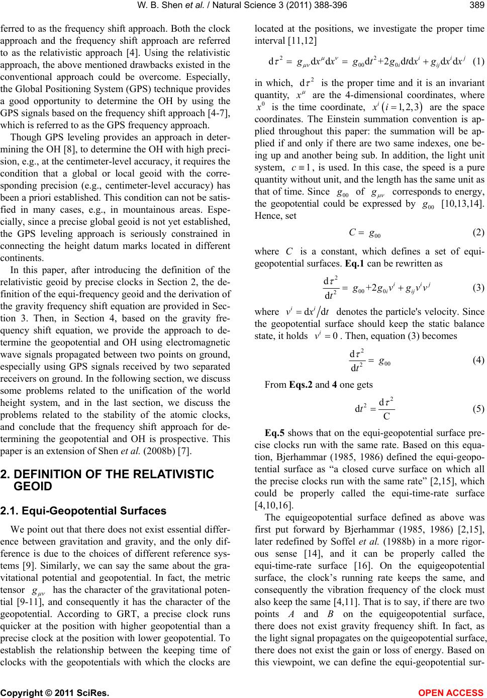 W. B. Shen et al. / Natural Science 3 (2011) 388-396 Copyright © 2011 SciRes. OPEN ACCESS 389 ferred to as the frequency shift approach. Both the clock approach and the frequency shift approach are referred to as the relativistic approach [4]. Using the relativistic approach, the above mentioned drawbacks existed in the conventional approach could be overcome. Especially, the Global Positioning System (GPS) technique provides a good opportunity to determine the OH by using the GPS signals based on the frequency shift approach [4-7], which is referred to as the GPS frequency approach. Though GPS leveling provides an approach in deter- mining the OH [8], to determine the OH with high preci- sion, e.g., at the centimeter-level accuracy, it requires the condition that a global or local geoid with the corre- sponding precision (e.g., centimeter-level accuracy) has been a priori established. This condition can not be satis- fied in many cases, e.g., in mountainous areas. Espe- cially, since a precise global geoid is not yet established, the GPS leveling approach is seriously constrained in connecting the height datum marks located in different continents. In this paper, after introducing the definition of the relativistic geoid by precise clocks in Section 2, the de- finition of the equi-frequency geoid and the derivation of the gravity frequency shift equation are provided in Sec- tion 3. Then, in Section 4, based on the gravity fre- quency shift equation, we provide the approach to de- termine the geopotential and OH using electromagnetic wave signals propagated between two points on ground, especially using GPS signals received by two separated receivers on ground. In the following section, we discuss some problems related to the unification of the world height system, and in the last section, we discuss the problems related to the stability of the atomic clocks, and conclude that the frequency shift approach for de- termining the geopotential and OH is prospective. This paper is an extension of Shen et al. (2008b) [7]. 2. DEFINITION OF THE RELATIVISTIC GEOID 2.1. Equi-Geopotential Surfaces We point out that there does not exist essential differ- ence between gravitation and gravity, and the only dif- ference is due to the choices of different reference sys- tems [9]. Similarly, we can say the same about the gra- vitational potential and geopotential. In fact, the metric tensor has the character of the gravitational poten- tial [9-11], and consequently it has the character of the geopotential. According to GRT, a precise clock runs quicker at the position with higher geopotential than a precise clock at the position with lower geopotential. To establish the relationship between the keeping time of clocks with the geopotentials with which the clocks are located at the positions, we investigate the proper time interval [11,12] 22 00 0 d dd d+2dddd iij iij xxg tgtxgxx (1) in which, 2 d is the proper time and it is an invariant quantity, are the 4-dimensional coordinates, where 0 is the time coordinate, 1, 2, 3 i xi are the space coordinates. The Einstein summation convention is ap- plied throughout this paper: the summation will be ap- plied if and only if there are two same indexes, one be- ing up and another being sub. In addition, the light unit system, 1c , is used. In this case, the speed is a pure quantity without unit, and the length has the same unit as that of time. Since 00 of corresponds to energy, the geopotential could be expressed by 00 [10,13,14]. Hence, set 00 Cg (2) where C is a constant, which defines a set of equi- geopotential surfaces. Eq.1 can be rewritten as 2 00 0 2 d +2 d iij iij gv gvv t (3) where dd ii vxt denotes the particle's velocity. Since the geopotential surface should keep the static balance state, it holds 0 i v . Then, equation (3) becomes 2 00 2 d d t (4) From Eqs.2 and 4 one gets 2 2d dC t (5) Eq.5 shows that on the equi-geopotential surface pre- cise clocks run with the same rate. Based on this equa- tion, Bjerhammar (1985, 1986) defined the equi-geopo- tential surface as “a closed curve surface on which all the precise clocks run with the same rate” [2,15], which could be properly called the equi-time-rate surface [4,10,16]. The equigeopotential surface defined as above was first put forward by Bjerhammar (1985, 1986) [2,15], later redefined by Soffel et al. (1988b) in a more rigor- ous sense [14], and it can be properly called the equi-time-rate surface [16]. On the equigeopotential surface, the clock’s running rate keeps the same, and consequently the vibration frequency of the clock must also keep the same [4,11]. That is to say, if there are two points and B on the equigeopotential surface, there does not exist gravity frequency shift. In fact, as the light signal propagates on the quigeopotential surface, there does not exist the gain or loss of energy. Based on this viewpoint, we can define the equi-geopotential sur-  W. B. Shen et al. / Natural Science 3 (2011) 388-396 Copyright © 2011 SciRes. OPEN ACCESS 390 face as follows [4,10,16]: the equigeopotential surface is such a closed curve surface on which there does not exist gravity frequency shift. The equigeopotential surface so defined may be properly called the equi-frequency sur- face [4,16]. 2.2. Relativistic Geoid In conventional geodesy, the geoid is defined as “the closed equi-geopotential surface nearest to the mean sea level” [1], which is referred to as the conventional geoid for convenience. In relativistic geodesy, based on the definition of the equi-time-rate surface, Bjerhammar (1985, 1986) defined the relativistic geoid as “the closed curve surface nearest to the mean sea level on which precise clocks run with the same rate” [2,15], which is properly referred to as the equi-time-rate geoid [4,10]. In fact, based on the defini- tion of the equi-time-rate surface, the relativistic geoid can be simply defined as the equi-time-rate surface nearest to the mean sea level. According to the relativistic definition, the geoid can be determined by using precise clocks. Combining Eqs.4 and 5 one can write down 12 12 00 1 ddd tg C (6) which gives rise to a clock’s running rate on an arbitrary equi-time-rate surface. Suppose the equi-time-rate geoid 0 S and an arbitrary equi-time-rate surface S are re- spectively given by the following equations: 00 0 00 C C (7) where 0 C and C are the geopotential constants on the equi-time-rate geoid 0 S and the equi-time-rate sur- face S, respectively. Then 12 12 00 dd, dd HH tCt C (8) and consequently we have 0 0 dd H H C tt C (9) where 0 dt and d t denote the clocks’ running rates (unit seconds) on the equi-time-rate geoid and the H- equi-time-rate surface that passes the point just above the datum point on the geoid with the OH, denoted by , respectively. It is noted that the difference between the relativistic geoid and the conventional geoid is about 0.5 cm [10,17]. Such a difference could be neglected in general applica- tions, but should be taken into account in high precise geoid determination. According to Eq.6 the geopotential value at an arbi- trary point on the Earth’s surface can be determined based on the clock transportation approach [3]. Though there are other approaches for time comparison between two separated clocks located at two stations, e.g., the GPS common-view approach and the approach of two-way time transfer by satellite [18], they provide the accuracy about parts of nanoseconds, and consequently they are too poor to determine a meaningful geopotential difference. In non-rela- tivistic geodesy, the measure- ments of the geopotentials are generally realized by combining gravimetry and leveling. The measurement procedure is very laborious, and the accumulated meas- urement error becomes larger and larger as the length of the measurement line increases. These drawbacks could be overcome by clock transportation approach. We note that the accuracy of determining the geopotentials by using precise clocks depends on the accuracies of the clocks. If the accuracy level of the atomic clocks is on the order of 10−16, the accuracy level of the determined geopotentials corresponds to the height difference of 1 meter. In recent years, the time and frequency science develop quickly. Atomic clocks with the stability level of 10−16 have been created [19-21]. It is noted that there are several study groups investigating the “optical fre- quency standard”, and significant results have been achieved [22-27]. They compared the different “optical frequency standards”, and found that all the stabilities are in the level of 10−18 to 10−19 [27]. Scientists predict that, in the near future, “optical clocks” with the stability of 10−18 could be realized. This will provide a firm foundation for determining the geopotential or OH at the centimeter level using clock transportation approach [3] or frequency shift approach (see Section 3). However, concerning the clock transportation ap- proach, at present, the atomic clocks available are very expensive, very heavy, and quite difficult for normal work during the transportation. Hence, only if portable, rela- tively cheap and precise clocks were created, one has to pursue other approaches to determine the geopotential differences. This is the motivation that the frequency shift approach was proposed [4,7]. 3. FREQUENCY SHIFT EQUATION OF ELECTROMAGNETIC SIGNALS On the equi-geopotential surface, an atomic clock’s running rate keeps the same, and consequently the fre- quency of an atomic clock must also keep the same [6,10-12]. Since a clock’s running rate is controlled by the vibration frequency, we can conclude that for arbi- trary two points and B at rest on a same equi- geopotential surface there does not exist electromagnetic signal’s frequency shift, which is referred to as the grav- ity (or geopotential) frequency shift. In virtue of this  W. B. Shen et al. / Natural Science 3 (2011) 388-396 Copyright © 2011 SciRes. OPEN ACCESS 391 viewpoint, an equi-geopotential surface could be defined as “a closed curve surface on which there does not exist gravity frequency shift” [4,6,10,16], which is referred to as the equi-frequency surface. Then, based on the definition of the equi-frequency surface the relativistic geoid could be defined as “the closed curve surface nearest to the mean sea level on which there does not exist gravity frequency shift”, which is referred to as the equi-frequency geoid [4]. Or, the relativistic geoid can be simply defined as the equi-frequency surface nearest to the mean sea level [4,6,10,16]. Based on the definition of the equi-frequ- ency geoid one can determine the relativistic geoid by measuring the gravity frequency shifts of electromag- netic signals. Since the frequency is inversely related to the period based on which the unit second is defined (see http://en. wikipedia.org/wiki/Second_unit), according to Eq.9 one has [6,10,12] 0 0 H H C f C (10) where 0 C and C are the geopotential constants cor- responding to the geoid and the H-equi-frequency geo- potential surface that passes the point just above the da- tum point on the geoid with the OH, H, respectively, 0 and are the atomic clocks’ frequencies on the equi-frequency geoid and the H-equi-frequency geopo- tential surface, respectively. By frequency shift observa- tions, 00H ff might be determined. Hence, based on Eq.10, if the geopotential constant 0 C on the geoid is determined, C can be determined. It is noted that, at least at present or in the near future, the equi-frequency geoid is more realizable than the equi-time-rate geoid [10]. At present, it is difficult to generally realize the comparisons between two separated clocks by clock transportation approach, due to the fact that precise atomic clock are very expensive for general usage. On the contrary, it is quite easy to generally real- ize the frequency shift observations, e.g., the generally used GPS observations. Suppose a light signal with frequency is emitted from point P and it is received at point Q. Because of the geopotential difference between these two points, the frequency of the received signal is not but . Based on Eq.4, the running rates of the atomic clocks P and Q at arbitrary two points on ground are given by the following equation 00 00 d d Q PQ g t tg (11) Based on the above equation one has 00 00 = 1 QP Q PP g ff fff ff fg (12) where f , Q f . In Eq.12, and Q are the frequencies at P and Q, respectively. Accurate to the order 2 V (V is the gravitational potential), 00 can be expressed as [10,11] 22 00 12 22122 VV WV (13) where WV is the classical Newtonian geopoten- tial, is the centrifugal force potential. Throughout this paper the definition of the geopotential in physical geodesy is applied: it always holds that 0W, which is different from the definition in physics. Combining Eqs. 12 and 13, accurate to W , one has QP fffW fWW (14) where W and Q W are the geopotentials at point P and Q, respectively. Eq.14 is the gravity frequency shift equation, which was confirmed by various physics ex- periments [28-32]. The frequency approach has special advantages com- pared to the clock transportation approach (Cf. Section 4). As mentioned before, concerning the OH determina- tion, clock transportation approach is difficult for gen- eral applications (Cf. Section 2.2). However, the gravity frequency shift between arbitrary two points P and Q on ground could be directly determined using GPS sig- nals, even these two points are located far away from each other (Cf. Section 4.2). Suppose the geopotential at point P is given, then from Eq.14 one can determine the geopotential at an arbitrary point Q by measuring the gravity frequency shift between P and Q, in virtue of the following equation QP WW (15) If the point P is chosen on the geoid, then one has (Shen et al., 2008a) 0Q WC (16) where 0 C is the geoid geopotential constant, the deter- mination of which could be found in e.g., Chao et al. (2007) [33]. Once 0 C is determined, the geopotential at an arbitrary point Q on the Earth’s surface can be deter- mined by using frequency shift observation method. The basic principle of measuring the frequency shift is stated in the sequel. Referring to Figure 1, set at point P an emitter which emits a signal with frequency and a receiver at point Q receives the emitted signal with frequency com- 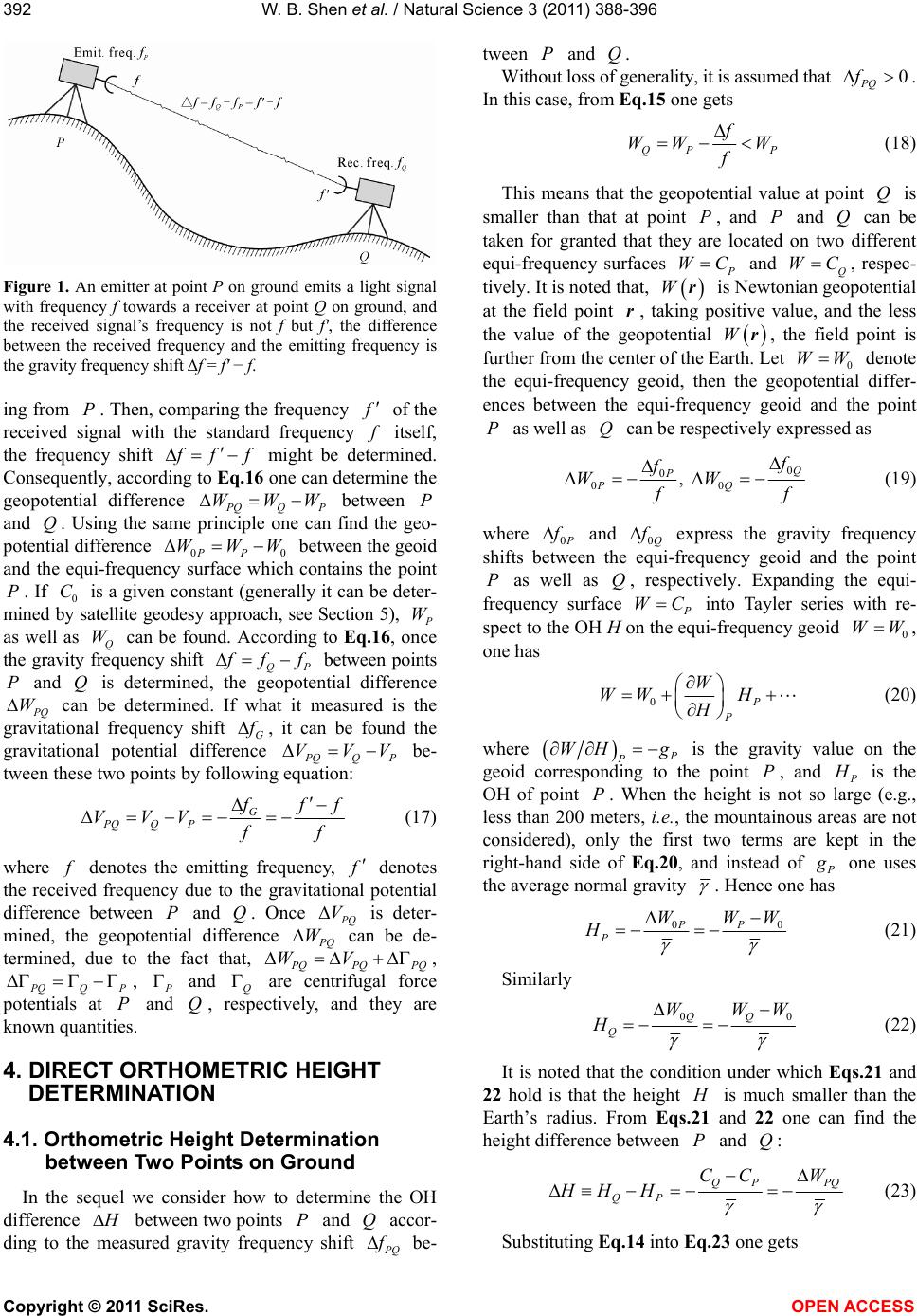 W. B. Shen et al. / Natural Science 3 (2011) 388-396 Copyright © 2011 SciRes. OPEN ACCESS 392 Figure 1. An emitter at point P on ground emits a light signal with frequency f towards a receiver at point Q on ground, and the received signal’s frequency is not f but f', the difference between the received frequency and the emitting frequency is the gravity frequency shift Δf = f' − f. ing from P. Then, comparing the frequency of the received signal with the standard frequency itself, the frequency shift ff might be determined. Consequently, according to Eq.16 one can determine the geopotential difference QQP WWW between P and Q. Using the same principle one can find the geo- potential difference 00PP WWW between the geoid and the equi-frequency surface which contains the point P. If 0 C is a given constant (generally it can be deter- mined by satellite geodesy approach, see Section 5), W as well as Q W can be found. According to Eq.16, once the gravity frequency shift QP ff between points P and Q is determined, the geopotential difference Q W can be determined. If what it measured is the gravitational frequency shift G , it can be found the gravitational potential difference QQP VVV be- tween these two points by following equation: G PQQ P f f VVV f (17) where denotes the emitting frequency, denotes the received frequency due to the gravitational potential difference between P and Q. Once Q V is deter- mined, the geopotential difference Q W can be de- termined, due to the fact that, QPQPQ WV, QQP , and Q are centrifugal force potentials at P and Q, respectively, and they are known quantities. 4. DIRECT ORTHOMETRIC HEIGHT DETERMINATION 4.1. Orthometric Height Determination between Two Points on Ground In the sequel we consider how to determine the OH difference between two points P and Q accor- ding to the measured gravity frequency shift Q be- tween P and Q. Without loss of generality, it is assumed that 0 PQ f . In this case, from Eq.15 one gets QP P f WW W f (18) This means that the geopotential value at point Q is smaller than that at point P, and P and Q can be taken for granted that they are located on two different equi-frequency surfaces WC and Q WC, respec- tively. It is noted that, Wr is Newtonian geopotential at the field point r, taking positive value, and the less the value of the geopotential Wr, the field point is further from the center of the Earth. Let 0 WW denote the equi-frequency geoid, then the geopotential differ- ences between the equi-frequency geoid and the point P as well as Q can be respectively expressed as 0 0 00 ,Q P PQ f WW f (19) where 0 and 0Q express the gravity frequency shifts between the equi-frequency geoid and the point P as well as Q, respectively. Expanding the equi- frequency surface WC into Tayler series with re- spect to the OH H on the equi-frequency geoid 0 WW , one has 0P P W WW H H (20) where P WH g is the gravity value on the geoid corresponding to the point P, and is the OH of point P. When the height is not so large (e.g., less than 200 meters, i.e., the mountainous areas are not considered), only the first two terms are kept in the right-hand side of Eq.20, and instead of one uses the average normal gravity . Hence one has 00PP P WWW H (21) Similarly 00QQ Q WWW H (22) It is noted that the condition under which Eqs .2 1 and 22 hold is that the height is much smaller than the Earth’s radius. From Eqs.21 and 22 one can find the height difference between P and Q: QP PQ QP CCW HH H (23) Substituting Eq.14 into Eq.23 one gets  W. B. Shen et al. / Natural Science 3 (2011) 388-396 Copyright © 2011 SciRes. OPEN ACCESS 393 1 H (24) From Eq.24 one can see that the accuracy of depends on that of , and consequently it is related to the stabilities of the frequencies of the emitter and re- ceiver. In theory, if the stabilities of the frequencies of the emitter and receiver are better than 10−18 (which is possible to be achieved because of quick development of time science, Cf. Section 2), the accuracy in determining the height difference between two different points could achieve the order of centimeter. Based on the above analysis one can see that, no matter what is determined, the geopotential difference (14), the gravitational poten- tial difference (17), or the height difference (24), the key problem is how to measure the gravity frequency shift and estimate the accuracy of . We note that the gra- vitational frequency shift can be determined if the grav- ity frequency shift is determined and vice versa. It should be emphasized that Eq.24 is only suitable to the non-rough areas. In the mountainous areas, Eq.2 0 should be kept to the second order of the height H. The details are referred to [6,17]. 4.2. OH Determination Using GPS Signals Referring to Figure 2, suppose an emitter is set on board a flying satellite (e.g., GPS satellite), which can emit electromagnetic wave signals with regular intervals. Then, by receiving the signals from the emitter simulta- neously at two points P and Q, one could determine the geopotential difference between P and Q, based on the gravity frequency shift Eq.14. Now, suppose the signal emitter E is set on board a satellite, and two signal receivers P and Q on ground receive the signals coming from E corresponding to an emitting time t. Further suppose the received frequen- cies of the signals corresponding to time t are recorded Figure 2. Two receivers at points P and Q on the Earth’s sur- face receive simultaneously the light signals with fre- quency f emitted on board a flying satellite S. by P and Q receivers in some way, respectively, i.e., and Q at t and Q t (P tt and Q tt, due to the delay of the signal propagation) are recorded by re- ceivers at P and Q, respectively. Note that the time t at which the signal is received by P receiver is generally different from the time Q t at which the signal is received by Q receiver. By comparing the received frequencies P f and Q f it could be determined the geopotential difference QQP WWW [4], which is just given by Eq.14 . One of the advantages by using the geopotential fre- quency shift approach lies in that a unified global height datum system could be established: two receivers lo- cated at two height datum points and B, which belong to two separated continents or islands, could si- multaneously receive the signals emitted by a satellite source emitter, and consequently the frequency shift between and B is determined; then, based on the geopotential frequency shift equation the geopotential difference as well as the OH difference between and B is determined. By such a way, the height datum of one continent (or island) could be connected to the height datum of another continent (or island). Then, a unified global height datum system might be established. In practical applications, however, the gravity fre- quency shift signals in GPS frequency observations are largely contaminated by other noise frequency shifts, which include the first-order Doppler frequency shift, ionosphere frequency shift, troposphere frequency shift, clock errors and random influences. To separate the gravity frequency shift signals from other noises is not so easy as generally imagined. Hence, to determine the geopotential or OH of an arbitrary point on ground, the key problem is how to draw the gravity frequency shift signals from the GPS frequency observations. The in- vestigations on this problem will be provided in a sepa- rated paper. 5. UNIFICATION OF THE WORLD ORTHOMETRIC HEIGHT DATUM SYSTEM Theoretically, the final determination of the geoid de- pends on the choice of constant 00 WC on the geoid. Given different 0 Ws, we get different equigeopotential surfaces. In practice, to determine the geoid, we always choose some tidal gauges’ average sea level as the da- tum (standard) of a local geoid. Theoretically, if 0 W is not determined properly, the real geoid will deviate from the datum. The key problem lies in that at this situation we still regard the datum as in consistency with the ge- oid. As a result, there will be a systematic error in the height system; and furthermore, since the mean sea level does not coincides with any equigeopotential surface  W. B. Shen et al. / Natural Science 3 (2011) 388-396 Copyright © 2011 SciRes. OPEN ACCESS 394 [10,34-41], various datums in the world are in fact lo- cated on different equigeopotential surfaces. This will give rise to the inconsistency of the world height system. If one chooses point A as the datum of the geoid, the geopotential constant 0 W on the geoid cannot be cho- sen arbitrarily but determined uniquely [10]. This is be- cause of two causes. One is in that to determine the ge- oid, a reference ellipsoid is needed. The normal potential 0 U on the surface of the ellipsoid is given a priori, or can be uniquely determined by the given parameters of the ellipsoid. No matter which method is chosen, 0 W is completely determined, since one should investigate gravity and normal gravity, geopotential and normal geopotential, etc., in the same system (a unified coordi- nate system). Another one lies in that to solve the boun- dary value problem we require that the gravitational part of W is regular at infinity. This condition (combining with the choice of the ellipsoid) will limit the variation of 0 W. Theoretically, we may suggest different methods to determine 0 W. The most basic method might be stated as follows [10]: Suppose we have chosen a refer- ence ellipsoid r E, e.g., WGS84 ellipsoid [42]. If a defi- nite shape of the ellipsoid is given (i. e. , given r E’s se- mimajor axis a and semiminor axis b), the normal geo- potential 0 U can be calculated theoretically, and con- sequently the geopotential constant 0 W on the geoid is determined (because of the condition that 00 UW ). However, a dilemma occurs: If 0 U is given, the r E’s semimajor and semiminor axises a and b are determined uniquely, but in this case we need to know 0 W a priori; inversely, if a and b are given, 0 U is determined uni- quely, but different a and b will introduce different 0 Us. Without previous knowledge, it is impossible to choose a and b so that 00 UW. The best way might be like this: one determines 0 U so that it app- roximates 0 W grad- ually. Hence, to precisely determine 0 W is a delicate matter [33,43]. Any error stemmed from 0 W will give rise to a systematic error to the geoid. In fact, How to precisely determine 0 W is an open problem. Once 0 Wis determined, the standard level geoid is determined. Then, using GPS frequency shift approach, we can unify the world height datum system. The basic principle is stated as follows. Suppose 0 W is precisely determined, e.g., with the accuracy of 1 cm level. Then, with the same accuracy level one can determine the OH of a datum point located at least in a relatively plain area with small OH. Then, the point is taken as the datum point of world height datum system. Referring to Figure 2, suppose the OH of a point P on ground is determined by leveling plus gravimetry approach between and P. Then, using GPS frequency shift approach one can de- termine the OH Q of an arbitrary point Q on ground. Since the point Q on ground is quite arbitrary, one can unify the world height datum system using the frequency shift approach. 6. DISCUSSIONS AND CONCLUSIONS According to the GRT, a precise (atomic) clock lo- cated at the position P with higher geopotential runs quicker than a precise clock located at the position Q with lower geopotential [12,44,45]. Equivalently, the vibration frequency of the clock at P is larger than that of the clock at Q. Then, the relativistic geoid can be defined based on the clock’s running rate, which is re- ferred to as the equi-time-rate geoid. In another aspect, the relativistic geoid can be defined based on the clock’s vibration frequency, or can be defined by the frequency shift equation, and so defined geoid is referred to as the equi-frequency geoid. The realization of the equi-freque- ncy geoid is based on the frequency shift approach, and the realization of the equi-time-rate geoid is based on the clock transportation approach. With clock transportation approach [3,46], the key problem is to compare two clocks located at different places by transporting portable clocks. Hence, one needs portable clocks to complete the comparisons. At present, though portable clocks with the stability better than 1 × 10⁻¹⁶ are not yet available, we may determine the geo- potential difference at the accuracy level of 1 m2·s−2 (equivalent to 0.1 m) between two separated points on ground by using clocks with the stability around 1 × 10⁻¹⁴ (Shen et al., 2009). The problem is whether the portable clocks with the stability 1 × 10⁻¹⁴ [3] for the aim of the transportation comparisons are available. With frequency shift approach, especially the GPS frequency shift approach [4,5,10,16,46], the key problem is to draw the frequency shift information from the fre- quency observations, which include other influences except for the gravity frequency shift. In fact, the GPS frequency observations include not only the gravity fre- quency shift, but also other noise frequency shifts such as the Doppler frequency shift, ionosphere frequency shift, troposphere frequency shift, etc. The noise fre- quency shifts should be removed from the observations. Obviously, after removing the noise frequency shifts, the accuracy in determining the OH depends on the stability of the time-keeping system. If the stability of the time-keeping system is better than 1 × 10⁻¹⁸, we can de- termine the OH with the accuracy of 1 cm. To directly determine the geopotential and OH using GPS signals, the GPS frequency shift approach is pro- spective. This is due to the fact that the time and fre- quency science develop very quickly, and clocks or time-keeping systems and portable clocks with the sta- bility better than 1 × 10⁻¹⁸ might be available in the near  W. B. Shen et al. / Natural Science 3 (2011) 388-396 Copyright © 2011 SciRes. OPEN ACCESS 395 future [22,27]. Then, a new era may come that the geo- metric position (coordinates) and the geopotential (as well as OH) could be simultaneously determined using GPS technique. 7. ACKNOWLEDGEMENTS This study is supported by National 863 Program of China (grant No. 2006AA12Z211) and the National Natural Science Foundation of China (grant No. 40637034). REFERENCES [1] Heiskanen, W.A. and Moritz, H. (1967) Physical geodesy. Freeman and Company, San Francisco. [2] Bjerhammar, A. (1985) On a relativistic geodesy. Bulletin Geodesique, 59, 207-220. doi:10.1007/BF02520327 [3] Shen, W.B., Ning, J.S., Liu, J.N. and Chao, D.B. (2009) A proposal on the test of general relativity by clock transportation experiments. Advances in Space Research, 43, 164-166. doi:10.1016/j.asr.2008.04.001 [4] Shen, W.B., Chao, D. and Jin, B. (1993) On the relativis- tic geoid. Bollettino di Geodesia e Scienze Affini, 52, 207-216. [5] Shen, W.B. and Ning, J. (2005) The application of GPS technique in determining the Earth’s potential field. Journal of GPS, 4, 268-276 doi:10.5081/jgps.4.1.268 [6] Shen, W.B., Ning, J. and Chao, D. (2008a) Relativity and relativistic gravimetry. Wuhan University Press, Wuhan. [7] Shen, W.B., Ning, J.S., Li, J.C., Liu, J.N. and Chao, D.B. (2008b) The concept of direct orthometric height deter- mination based on frequency shift equation. International Conference on Earth Observation Data Processing and Analysis, Wuhan, 29 December 2008, 1-8. [8] Moritz, H. (2000) Molodensky’s theory and GPS. Mitteil. Geod. Graz Technology University, Graz. [9] Shen, W.B. (1996) On the separability of gravitation and inertia according to general relativity. Dissertation, Graz Technical University, Graz. [10] Shen, W.B. (1998) Relativistic physical geodesy. Graz Technical University, Graz. [11] Soffel, M.H. (1989) Relativity in astrometry, celestial mechanics and geodesy. Springer-Verlag, Berlin. [12] Weinberg, S. (1972) Gravitation and cosmology. John Wiley & Sons, New York. [13] Soffel, M.H., Herold, H., Ruder, H. and Schneider, M. (1988) Relativistic geodesy: The concept of asymptoti- cally fixed reference frames. Manu. Geod., 13, 139-142. [14] Soffel, M.H., Herold, H., Ruder, H. and Schneider, M. (1988b) Relativistic theory of gravimetric measurements and definition of the geoid. Manu. Geod., 13, 143-146. [15] Bjerhammar, A. (1986) Relativistic geodesy. NOAA Technical Report NOS 118 NGS 36, Rockville. [16] Shen, W.B., Chao, D. and Jin, B. (1994) The concept and application of the equi-frequency geoid. Journal of Wu- han Technical University, 19, 232-238. [17] Shen, W.B., Ning, J., Li, J. and Chao, D. (2004) On the relativistic geopotential and relativistic geoid. Journal of Wuhan University (Information Science), 29, 897-900. [18] Hanson, D.W. (1989) Fundamentals of two-way time transfer by satellite. 43rd Annual Frequency Control Symposium, 31 May - 2 June 1989, pp. 174-178. doi:10.1109/FREQ.1989.68861 [19] Heavner, T. P., Jefferts, S.R., Donley, E.A., et al. (2005a) NIST-F1: Recent improvements and accuracy evaluations. Metrologia, 42, 411-422. doi:10.1088/0026-1394/42/5/012 [20] Heavner, T.P., Jefferts, S.R., Donley, E.A., et al. (2005b) Recent improvements in NIST-F1 and a resulting accu- racy of 0.61 × 10⁻¹⁵. IEEE Transactions on Instrumenta- tion and Measurement, 54, 842-845. doi:10.1109/TIM.2005.843812 [21] Parker, T.E., Heavner, T.P., Jefferts, S.R., et al. (2005) Operation of the NIST-F1 caesium fountain primary fre- quency standard with a maser ensemble, including the impact of frequency transfer noise. Metrologia, 42, 423- 430. doi:10.1088/0026-1394/42/5/013 [22] Jones, D.J. (2000) Carrier-envelope phase control of femtosecond mode-locked lasers and direct optical fre- quency synthesis. Science, 288, 635-638. doi:10.1126/science.288.5466.635 [23] Reichert, J., Niering, M. and Holzwarth, R. (2000) Phase coherent vacuum-ultraviolet to radio frequency com- parison with a mode-locked laser. Physical Review Let- ters, 84, 3232-3235. doi:10.1103/PhysRevLett.84.3232 [24] Diddams, S.A., Jones, D.J., Ye, J., et al. (2000) Direct link between microwave and optical frequencies with a 300 THz femtosecond laser comb. Physical Review Let- ters, 84, 5102-5105. doi:10.1103/PhysRevLett.84.5102 [25] Diddams, S.A., Udem, T., Bergquist, J.C., et al. (2001) An optical clock based on a single trapped 199Hg+ ion. Science, 293, 825-828. doi:10.1126/science.1061171 [26] Ye, J., Tai, H.Y. and John, L.H. (2000) Accuracy com- parison of absolute optical frequency measurement be- tween harmonic-generation synthesis and a frequency- division femtosecond comb. Physical Review Letters, 85, 3797-3800. doi:10.1103/PhysRevLett.85.3797 [27] Ma, L., Bi, Z., Bartels, A., et al. (2004) Optical fre- quency synthesis and comparison with uncertainty at the 10−19 level. Science, 303, 1843-1845. doi:10.1126/science.1095092 [28] Pound, R.V. and Snider, J.R. (1965) Effect of gravity on gamma radiation. Physical Review, 140B, 788. doi:10.1103/PhysRev.140.B788 [29] Vessot, R.F.C., Levine, M.W., Mattison, E.M., et al. (1980) Test of relativistic gravitation with a space-borne hydrogen maser. Physical Review Letters, 45, 2081-2084. [30] Katila, T. and Riski, K.J. (1981) Measurement of the interaction between electromagnetic radiation and gravi- tational field using Zn67 Mössbauer spectroscopy. Phys- ics Letters, 83A, 51-54. [31] Turneaure, J.P., Will, C.M., Farrel, B.F., et al. (1983) Test of principle of equivalence by a null gravitational red- -shift experiment. Physical Review D, 27, 1705-1714. doi:10.1103/PhysRevD.27.1705 [32] Bauch, A. and Weyers, S. (2002) New experimental limit on the validity of local position invariance. Physical Re- view D, 65, 1-4. doi:10.1103/PhysRevD.65.081101 [33] Chao, D., Shen, W.B. and Wang, Z. (2007) The possibil- ity and method investigations on the determination of the global centimeter level geoid. Acta Geodaetica et Carto-  W. B. Shen et al. / Natural Science 3 (2011) 388-396 Copyright © 2011 SciRes. OPEN ACCESS 396 graphica Sinica, 36, 370-376. [34] Sturges, W. (1972) Comments on ocean circulation with regard to satellite altimetry. Sea Surface Topography from Space, Vol. 2, Tech. Rep. ERL228-AOML7-2, The National Oceanic and Atmospheric Administration, Boulder. [35] Sturges, W. (1974) Sea level slope along continental boundaries. Journal of Geophysical Research, 79, 825. doi:10.1029/JC079i006p00825 [36] Hamon, B.V. and Greig, M.A. (1972) Mean sea level in relation to geodetic land leveling around Australia. Journal of Geophysical Research, 77, 7157. doi:10.1029/JC077i036p07157 [37] Fischer, I. (1975) Does mean sea level slope or down toward north? Bulletin Geodesique, 49, 17. doi:10.1007/BF02523939 [38] Rapp, R.H. (1988) The geoid definition and determina- tion. OSU Rep. 325. [39] Torge, W. (1989) Gravimetry. Walfer de Cruyter, Berlin. [40] Vanicek, P. and Krakiwsky, E. (1986) Geodesy: The concepts. 2nd Edition, North-Holland Pub. Co., Amster- dam. [41] Rapp, R.H. and Balasubramania, X. (1992) A conceptual formulation of a world height system. OSU Rep. No. 421. [42] WGS84, 2011. http://en.wikipedia.org/wiki/World_Geodetic_System [43] Grafarend, E.W. (1994) What is a geoid? In: Vanicek, P., Christou, N.T. Eds., Geoid and Its Geophysical Interpre- tations, CRC Press, London. [44] Misner, C.W., Thorne, K.S. and Wheeler, J.A. (1973) Gravitation. Freeman and Company, San Francisco. [45] Will, C.M. (1993) Theory and experiment in gravita- tional physics. Cambridge University Press, Cambridge. [46] Brumberg, V.A. and Groten, E. (2002) On determination of height by using terrestrial clocks and GPS signals. Journal of Geodesy, 76, 49-54. doi:10.1007/s001900100219
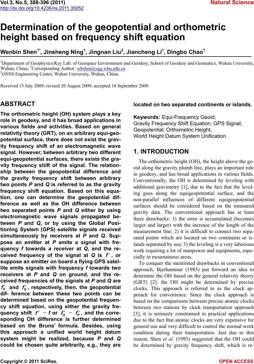
|