Int. J. Communications, Network and System Sciences, 2011, 4, 304-312
doi:10.4236/ijcns.2011.45035 Published Online May 2011 (http://www.SciRP.org/journal/ijcns)
A New On-Line/Off-Line Adaptive Antenna Array
Beamformer for Tracking the Mobile Targets
Shahriar Shirvani-Moghaddam1, Mahyar Shirvani-Moghaddam2
1Digital Communications Signal Processing Research Lab., Faculty of Electrical and Computer Engineering,
Shahid Raj aee Te acher Traini ng Uni v ersity, Tehran , Ira n
2Telecommunicat i on Labor atory, School of El ect ri cal and Information, Uni versit y of Sy dney, Sydney, Austral ia
Received February 26, 2011; revised April 7, 2011; accepted April 23, 2011
Abstract
An adaptive antenna array system adjusts the main lobe of radiation pattern in the direction of desired signal
and points the nulls in the direction of undesired signals or interferers. The essential goal of beamforming is
to reduce the complexity of weighting process and to decrease the time needed for adjusting the antenna ra-
diation pattern. In this article a new adaptive weighting algorithm is proposed for both least mean squares
(LMS) and constant modulus (CM) algorithms. It is appropriate and applicable for antenna array systems
with moving targets and also mobile applications as well as sensor networks. By predicting the relative ve-
locity of source, the next location of the source will be estimated and the array weights will be determined
using LMS or CM algorithm before arriving to the new point. For the next time associated to the new sam-
pling point, evaluated weights will be used. Furthermore, by updating these weights between two consecu-
tive times the effects of error propagation will be eliminated. Therefore, in addition to reduction in computa-
tional complexity at the time of weight allocation, relatively accurate weight allocation can be obtained. Si-
mulation results of this investigation show that the angular error related to both LMS-based and CM-based
algorithms is less than the conventional LMS and CM algorithms at different signal to noise ratios (SNRs).
On the other hand, due to considering off-line process, online computational complexity of new algorithms is
slightly low with respect to previous ones.
Keywords: Beamforming, Adaptive Antenna Array, LMS, CM, Training-Based, Blind
1. Introduction
Growth in wireless technologies and users’ demands,
lead us to extend these systems in rural and urban areas,
indoor and outdoor environments, short-range as well as
long-range applications and then optimizing them for
long term scheduling. During these two decades, appro-
priate beamforming and concentrating radiated power in
specific directions using antenna (sensor) arrays are been
so attractive [1]. In digital beamforming, instead of hard-
ware changes, major part of processing is done by digital
processors in intermediate frequency (IF) or baseband.
This type of processing increases the flexibility and re-
duces the size of the system. By appropriate beamform-
ing at the transmitter, receiver or both, we can reach to
higher receiving power, better signal to noise plus inter-
ference ratio (SNIR), and lower bit error rate (BER).
There are two major techniques for forming the radia-
tion pattern of antenna arrays, fixed beam and adaptive
processing [2-4]. As shown in fixed-beam methods, sta-
tistically optimum weight vectors for beamforming can
be calculated by the Wiener solution. However, knowl-
edge of the asymptotic second-order statistics of the sig-
nal and the interference-plus-noise should be assumed.
These statistics are usually not known but with the as-
sumption of ergodicity, where the time average equals
the ensemble average, they can be estimated from the
available data. For time-varying signal environments,
such as wireless cellular communication systems, statis-
tics change with time as the source and interferers move
around the cell. For the time-varying signal propagation
environment, a recursive update of the weight vector is
needed to track a moving mobile or terminal so that the
spatial beam filtering will adaptively steer to the target

S. SHIRVANI-MOGHADDAM ET AL. 305
mobile’s time-varying direction of arrival (DOA), thus
resulting in optimal transmission/reception of the desired
signal. To solve the problem of time-varying statistics,
weight vectors are typically determined by adaptive al-
gorithms which adapt to the changing environment [5,6].
In adaptive beamforming, according to the system condi-
tion, antenna array and its pattern will be adjusted dy-
namically. Thus, in this system, there is a processing unit.
Types of antennas, their configurations and forwarding
information to the processor depend on the application.
There are two different methods, based on training
sequences and blind estimation, for adaptive weighting
of antenna array elements. In training based methods one
reference signal is required and they do not need to know
the location of signal source and hence they will be con-
verged faster than blind algorithms. In contrast, in blind
methods, the only thing that is required is the DOA of
the main signal (source) and other information should be
obtained from received signal [7,8].
In recent years different research works have been
done in the field of smart antenna and digital beamform-
ing. Reviewing these works shows that the effect of the
direction and velocity of the source has not been consid-
ered seriously and if it has been used, calculations and
computational complexity in the weighting step have
been increased. For example, in [9], authors propose a
normalized least mean square (NLMS) adaptive algo-
rithm that incorporates a direction of arrival detection
criterion. Simulation results of this investigation show
that the number of NLMS adapted parameters can be
reduced by this method. This method provides signifi-
cantly improved convergence and tracking capabilities.
Authors in [10] shows that by using adaptive beam-
forming technique based on maximum likelihood estima-
tion (MLE) robustness of algorithms against the effects
of incorrect direction of arrival (DOA) estimation can be
increased. In [11], the performance of an autoregressive
(AR), super resolution beamforming technique is ana-
lyzed and compared with other high resolution methods.
The AR parameters in [11] are determined adaptively
using the least mean square (LMS) algorithm.
Practical design of a smart antenna system based on
DOA estimation and adaptive beamforming is the subject
of [12]. In [12] DOA estimation is based on multiple
signal classification (MUSIC) algorithm and adaptive
beamforming is achieved using the LMS algorithm.
In [13] the performance of LMS and recursive least
square (RLS) algorithms for smart antennas in a wide-
band code division multiple access (W-CDMA) mobile
communication environment is discussed. Furthermore,
beamforming algorithms based on NLMS and matrix
inverse (MI) are processed in [14]. In [15] a matrix in-
version normalized least mean square (MI-NLMS) adap-
tive beamforming algorithm is described with tracking.
Simulation results of this method show that BER im-
provement is proportional to the number of antenna ele-
ments employed in the antenna array. Performance of
constant modulus (CM), LMS, and RLS algorithms are
discussed in [16] and a systematic comparison between
them is obtained. The linearly constrained constant mod-
ulus algorithm (LCCMA) is the subject of [17]. In [18,
19], the performance of blind adaptive beamforming
algorithms for smart antennas in realistic environments
with a constrained constant modulus (CCM) design cri-
terion is described and used for deriving a RLS type op-
timization algorithm. Ref. [20] shows a systematic com-
parison of the performance of different modified blind
adaptive beamforming algorithms based on CCM. Two
of them use adaptive step size mechanisms, in the sto-
chastic Gradient (SG) algorithm for adjusting the step
size and other one uses RLS type optimization algorithm
which is replaced by inverse of correlation matrix instead
of step size.
In the present article, by using LMS and CM algo-
rithms, a new simple method for predicting the direction
and velocity of source has been proposed. In comparison
with other algorithms and also previous research works,
it adds no additional calculations and complexity in the
time of radiation pattern shaping (denoted as online
process) and the main calculations are done by a separate
processor in the time intervals between two consecutive
times (denoted as offline process). Another advantage of
the proposed algorithm is the simplicity of the estimation
of the DOA related to the conventional DOA algorithms.
The rest of this paper is organized as follow. In Sec-
tion 2, some important basic notes about adaptive an-
tenna array systems are illustrated and two well-known
algorithms, LMS and CM, are discussed in detail. Sec-
tion 3 introduces the new proposed algorithm which is
based on prediction the next location of source and doing
the required processes in two steps, on-line as well as
off-line. In addition to simulation assumptions and re-
lated flowchart, the simulation results of conventional
LMS and CM as well as proposed ones are described in
Section 4. Finally, Section 5 concludes this article.
2. Adaptive Antenna Array Systems
Antenna array is a set of antennas connected to a digital
signal processor which are used for transmitting and re-
ceiving electromagnetic waves in coherent manner. Each
antenna is an element of array. The transmitting beam in
transmitter and/or receiving pattern in receiver can be
formed using a processor in based-band by combining the
array element signals. This process is called digital
beamforming. Two most important parameters for deter-

S. SHIRVANI-MOGHADDAM ET AL. 306
mining the radiation pattern of antenna arrays are the
weighting method in reception and the type of feeding the
elements in transmission. Hence some adaptive methods
have been proposed for producing appropriate radiation
patterns.
Assume a k-element antenna array as depicted in Fig-
ure 1. In order to obtain an appropriate radiation pattern,
signals of array elements should be multiplied in the
complex weights and weighted signals should be com-
bined linearly. This process is called weighting. After
receiving the signal at element Ant1, it is multiplied with
weight w1 which modify the amplitude and phase of input
signal. Then, according to (1), a linear system combines
these weighted signals to create output signal.
 


112 2kk

y
nwxnwxn wxn  (1)
The main feature of antenna array is the ability to sep-
arate signals in space. Signal separation in space means
adjusting the main lobe of antenna in the direction of de-
sired signal (main signal) and nulls in the direction of
undesired signals (interferers). Therefore, input and out-
put signals should be compared. In this investigation,
LMS and CM algorithms are considered to find the best
weights of antenna array system.
2.1. LMS Algorithm
LMS algorithm uses minimum mean square error
(MMSE) criterion for weight estimation. In MMSE, if
is considered as a function of , this func-
tion has only one minimum (bowl-shape surface). The
location of this minimum can be determined by solving
the Wyner optimization equation. Figure 2 shows the
bowl- shape surface for two-weight function.


2
Et 

w
It is also known that the gradient of this surface, i.e.,
, is a vector directed to the maximum point
of surface with minimum distance. Therefore, it will be
moved to the minimum point with minimum distance, if
it is altered the weights according to the negative slope
of this vector. This method is called steepest-descent.
This is the best choice to move toward the minimum
point. This fact can be proven by stronger mathematical
methods.


2
wEt
 

One of the interesting features of this method is that
when we are close to the minimum point, the slope of
gradient vector is high, and by increasing the distance to
this point the slope of this vector is decreased. This fea-
ture avoids weight oscillation and instability due to varia-
tions of time variant channels.
According to the above mentioned descriptions, it can
be summarized as follow:


2
d
dw
wEt
t
  
Figure 1. Adaptive antenna array structure.
Figure 2. The surface of a two-weight array system.








22
2HH EtEdt wrwR  w

 (3)

d2
d
wrRw
t



 (4)






 

*, H
rEdtxt RExtxt

(5)
 

 
*
d2,
d
wExtttyt dt
t
   (6)
where

is a coefficient that determines the conver-
gence speed of the algorithm, represents reference
signal, and

dt
H
indicates Hermitian conjugate.
In (6) we use the real-time value instead of average
value. This simplification is shown in (7).
 
*
d2
d
w
x
t
t
  

(2) t (7)

S. SHIRVANI-MOGHADDAM ET AL. 307

For discrete-time case, derivations can be substituted
with subtraction as follow:
 
*
1wnwnxn n    (8)
Equation (8) shows that using real-time approximation
instead of expected value can introduce an iterative algo-
rithm with simpler implementation. However, some notes
should be considered about convergence speed. The sur-
face is the bowl-shaped which its shape is
determined with eigen values of output correlation ma-
trix of array. The crater of bowl will be too open and the
slope of its walls will be small, if this eigen values are far
together. Therefore, the convergence speed will be de-
creased.


2
Et 
2.2. CM Algorithm
In some techniques that modulate information in phase
(such as M-ary phase shift keying (MPSK)) or frequency
(such as M-ary frequency shift keying (MFSK)), the en-
velope of signal remains constant. The CM algorithm is
first proposed by Godard and it uses this constant enve-
lope feature. By calculating this envelope, adaptive
beamforming algorithm can be managed.
CM algorithm uses a cost function, named as diffrac-
tion function of order p, and after minimization, the op-
timum weights can be obtained. The Godard’s cost func-
tion is shown in (9).
 

2q
p
p
JnE ynR






(9)
where are equal to 1 or 2. Godard showed that if , pq
p
R is defined as in (10), the slope of the cost function
will be zero.




2
p
pp
Esn
REsn  (10)
where

s
n is the memoryless estimation of


y
n and
then the estimation error is:
 


2
p
p
p
nynyn Ryn 

 (11)
If we assume that , the cost function has the
form:
1p
 


2
1
JnE ynR


(12)




2
1
Esn
REsn  (13)
By rewriting the error signal in (11), (14) can be de-
rived.
 

yn
nynyn
  (14)
Updating equation of weights is:
   
*
1
11wnwny nxn
yn


 



(15)
It has been shown that the fastest convergence is ob-
tained by using 1p

.
3. New On-Line/Off-Line Proposed Method
In our proposed algorithm, according to the direction and
the velocity of the main signal source, new location of
user will be estimated. Also the weights of array will be
determined using LMS or CM before arriving at the es-
timated source location. When source reaches to the new
point, the antenna array uses these weights and regulates
the radiation pattern. For avoiding the error propagation,
it is essential that the exact location of the source be de-
termined and array weights be updated at the next step.
Details of the steps of new proposed algorithm are illus-
trated below:
1) Applying the weighting algorithm (LMS or CM) for
first two points and determining the direction of arrival
in two points 1

and 2

, and also obtaining the proper
weights. For example, in an 8-element uniform linear
array (ULA), and
.
11
24
,,w1214 15 16 17 18
, ,,,,,ww wwwww
, w ww
13
,w
,, w
21 2223
,,www 25 262728
2) Predicting the next location of the source (

or
eq

) by using the previous locations of the source. The
relative velocity has some effects on the value of the
angular locations 1 and 2. In this paper the direction of
the source motion has considered in the simulations.
Figure 3 shows two cases. If the source moves parallel
to main axis of array, according to (16) the new angular
location can be found.
21 2
2
2
vv
 
1




  (16)
3) Finding the proper weights
12345678
for adjusting the radiation
pattern in the direction of
,,,,,,,wwwwwwww

or eq

according to
weighting algorithm (LMS or CM).
4) Forming the radiation pattern according to the esti-
mated weights in step 3.
5) Finding the exact angular location (

or eq

) by
using LMS or CM algorithm in the time interval between
two sampling points (to avoid error propagation). Then
determining the new relative velocity of the source.
6) Going to step 2 and doing the steps 2 to 5.

S. SHIRVANI-MOGHADDAM ET AL. 308
Figure 3. Movement path of the source respect to main axis
of the array. (a) Parallel; b) With nonzero angle.
These 6 steps are summarized as a simulation flow-
chart in Figure 4.
It can be seen that except first and second points, the
other steps of new LMS-based and CM-based algorithms
are done in the time interval between two sampling
points. Therefore in each beamforming step, radiation
pattern just will be activated and other processes are
off-line. Table 1 shows the off-line and online processes
of conventional and new proposed on-line/off-line beam-
formers.
4. Simulations
In this section, first numerical results of LMS algorithm
at different SNRs for three cases, noisy channel, channel
with one interferer, and channel with two interferers in
both conventional and new proposed beamformers are
shown. Second, numerical results belong to simulation of
CM algorithm at different SNRs for three above men-
tioned channels in both conventional and new proposed
beamforming algorithms are illustrated. Here, the accu-
racy of source angle detection is the performance metric
and different simulations are done by changing the angle
of source signal in the interval of [−80˚, 80˚].
All simulations are run in MATLAB 7.5 package.
Required number of iterations to access acceptable re-
sults is 1000. Three scenarios, pure noisy, one interfer-
ence signal with angle of zero, and two interference sig-
nals in 0 and −40 degrees in 8-element uniform linear
antenna array are simulated.
Signal source moves in a defined path with constant
velocity. Three paths are considered, parallel to array, in
the direction of nonzero angle with array, and random
walk with constant velocity. In all simulations, average
relative angular velocity is less than 5 degrees in second
and signals are modulated using minimum shift keying
(MSK) method.
Finding antenna array weights using weighting
algorithm (LMS or CM) for two first points
Finding antenna array weights using weighting
algorithm (LMS or CM) for predicted location
Forming the antenna pattern according to the
weights for predicted location
Doing the Beamforming algorithm (LMS or CM)
at new sampling point and finding the exact
location of source
Predicting new location using a simple linear
predictor
Generating random sequences
(Trainings and data)
Output
Figure 4. Simulation flowchart of proposed on-line/off-line
beamformer.
Table 1. Required off-line and on-line processes for both
conventional and new proposed be amfor mer s.
Process Proposed
Beamformer Conventional Beamformer
Off-line
- Estimating the velocity
- Updating the predicted loca-
tion of source
- Finding the weights associ-
ated to the next location us-
ing LMS or CM
-
On-line - Antenna beamforming accor-
ding to calculated weights in
off-line phase
- Finding the appropriate
weights according to
LMS or CM.
- Applying the weights to
form the antenna pat-
tern
In Figure 5 the angular error of both conventional and
proposed LMS-based beamformers at different SNRs in
the case of noisy channel is shown. As depicted in this
figure, the angular accuracy of proposed algorithm is
very similar to conventional algorithm. Also Figures 6
and 7 show the angular error of two above mentioned
beamformers in terms of SNR in the 1-interference and
2- interference channels, respectively.
Figures 8, 9 and 10 show te angular error of both con- h

S. SHIRVANI-MOGHADDAM ET AL. 309
(a) (b)
Figure 5. Angular error of LMS-based beamformers in a noisy channel. (a) Conventional; (b) Proposed on-line/off-line.
(a) (b)
Figure 6. Angular error of LMS-based beamformers in the case of one interferer. (a) Conventional; (b) Proposed on-line/
off-line.
(a) (b)
Figure 7. Angular error of LMS-based beamformers in the case of two interferers. (a) Conventional; (b) Proposed on-line/
off-line.

S. SHIRVANI-MOGHADDAM ET AL. 310
(a) (b)
Figure 8. Angular error of CM-based beamformers in a noisy channel. (a) Conventional; (b) Proposed on-line/off-line.
(a) (b)
Figure 9. Angular error of CM-based beamformers in the case of one interferer. (a) Conventional; (b) Proposed on-line/
off-line.
(a) (b)
Figure 10. Angular error of CM-based beamformers in the case of two interferers. (a) Conventional; (b) Proposed on-line/
ff-line. o

S. SHIRVANI-MOGHADDAM ET AL. 311
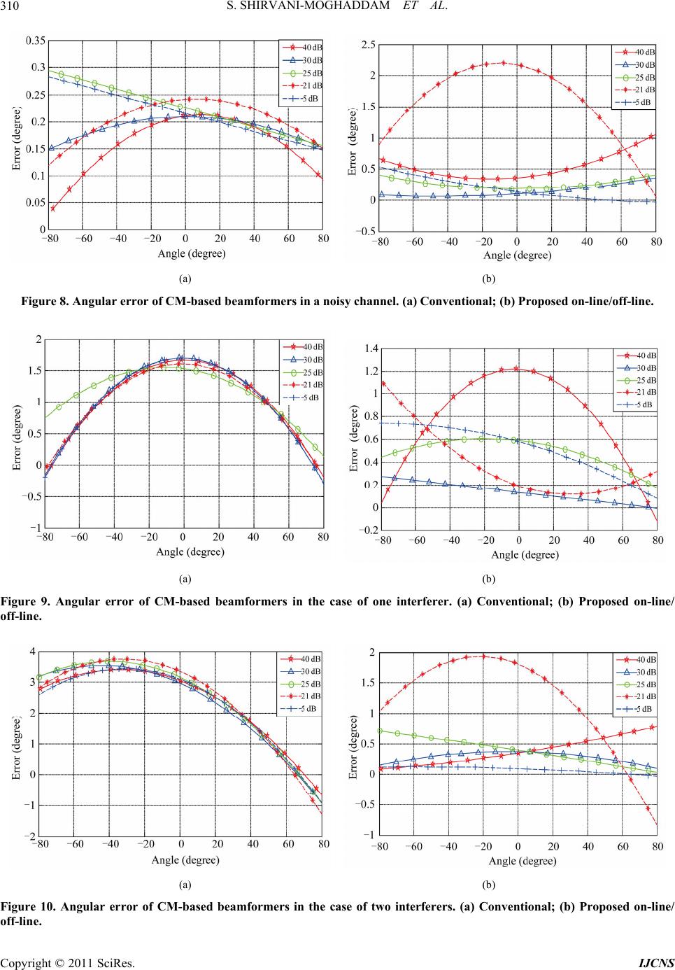
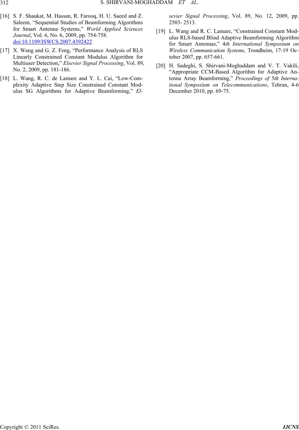
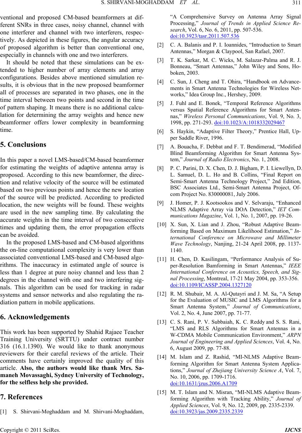
ventional and proposed CM-based beamformers at dif-
ferent SNRs in three cases, noisy channel, channel with
one interferer and channel with two interferers, respec-
tively. As depicted in these figures, the angular accuracy
of proposed algorithm is better than conventional one,
especially in channels with one and two interferers.
It should be noted that these simulations can be ex-
tended to higher number of array elements and array
configurations. Besides above mentioned simulation re-
sults, it is obvious that in the new proposed beamformer
all of processes are separated in two phases, one in the
time interval between two points and second in the time
of pattern shaping. It means there is no additional calcu-
lation for determining the array weights and hence new
beamformer offers lower complexity in beamforming
time.
5. Conclusions
In this paper a novel LMS-based/CM-based beamformer
for estimating the weights of adaptive antenna array is
proposed. According to this new beamformer, the direc-
tion and relative velocity of the source will be estimated
based on two previous points and hence the new location
of the source will be predicted. According to predicted
location, the new weights will be found. These weights
are used in the new sampling time. By calculating the
accurate weights in the time interval of two consecutive
times and updating them, the error propagation effects
can be avoided.
In the proposed LMS-based and CM-based algorithms
the on-line computational complexity is very lower than
associated conventional LMS-based and CM-based algo-
rithms. The inaccuracy in estimated angle of source is
less than 1 degree at pure noisy channel and less than 2
degrees in the channel with one and two interfering sig-
nals. This algorithm can be used for tracking in radar
systems and sensor networks and also regulating the ra-
diation pattern in mobile applications.
6. Acknowledgements
This work has been supported by Shahid Rajaee Teacher
Training University (SRTTU) under contract number
316 (16.1.1390). We would like to thank anonymous
reviewers for their careful reviews of the article. Their
comments have certainly improved the quality of this
article. Also, the authors would like thank Mrs. Sa-
maneh Mova ssaghi, Sydney University of Technology,
for the selfless help she provided.
7. References
[1] S. Shirvani-Moghaddam and M. Shirvani-Moghaddam,
“A Comprehensive Survey on Antenna Array Signal
Processing,” Journal of Trends in Applied Science Re-
search, Vol. 6, No. 6, 2011, pp. 507-536.
doi:10.3923/tasr.2011.507.536
[2] C. A. Balanis and P. I. Ioannides, “Introduction to Smart
Antennas,” Morgan & Claypool, San Rafael, 2007.
[3] T. K. Sarkar, M. C. Wicks, M. Salazar-Palma and R. J.
Bonneau, “Smart Antennas,” John Wiley and Sons, Ho-
boken, 2003.
[4] C. Sun, J. Cheng and T. Ohira, “Handbook on Advance-
ments in Smart Antenna Technologies for Wireless Net-
works,” Idea Group Inc., Hershey, 2009.
[5] J. Fuhl and E. Bonek, “Temporal Reference Algorithms
versus Spatial Reference Algorithms for Smart Anten-
nas,” Wireless Personal Communications, Vol. 9, No. 3,
1998, pp. 271-293. doi:10.1023/A:1018332029467
[6] S. Haykin, “Adaptive Filter Theory,” Prentice Hall, Up-
per Saddle River, 1996.
[7] A. Bouacha, F. Debbat and F. T. Bendimerad, “Modified
Blind Beamforming Algorithm for Smart Antenna Sys-
tem,” Journal of Radio Electronics, No. 1, 2008.
[8] P. C. Parini, D. X. Chen, D. J. Bigham, P. I. Liewellyn, D.
L. Samuel, D. L. Ho and B. Collins, “Final Report on
Semi-Smart Antenna Technology Project,” 2nd Edition,
BSC Associates Ltd., Semi-Smart Antenna Project, Of-
com Project No. 830000081, July 2006.
[9] J. Homer, P. J. Kootsookos and V. Selvaraju, “Enhanced
NLMS Adaptive Array via DOA Detection,” IET Com-
munications Magazine, Vol. 1, No. 1, 2007, pp. 19-26.
[10] X. Sun, X. Lian and J. Zhou, “Robust Adaptive Beam-
forming Based on Maximum Likelihood Estimation,” In-
ternational Conference on Microwave and Millimeter
Wave Technology, Nanjing, 21-24 April 2008, pp. 1137-
1140.
[11] H. Chen, D. Kasilingam, “Performance Analysis of Su-
per-Resolution Bamforming in Smart Antennas,” IEEE
International Conference on Acoustics, Speech, and Sig-
nal Processing, Montreal, 17-21 May 2004, pp. 353-356.
doi:10.1109/ICASSP.2004.1327120
[12] R. M. Shubair, M. A. Al-Qutayri and J. M. Sa, “A Setup
for the Evaluation of MUSIC and LMS Algorithms for a
Smart Antenna System,” Journal of Communications,
Vol. 2, No. 4, June 2007, pp. 71-77.
[13] C. S. Rani, P. V. Subbaiah, K. C. Reddy and S. S. Rani,
“LMS and RLS Algorithms for Smart Antennas in a
W-CDMA Mobile Communication Environment,” ARPN
Journal of Engineering and Applied Sciences, Vol. 4, No.
6, August 2009, pp. 77-88.
[14] M. Islam and Z. Rashid, “MI-NLMS Adaptive Beam-
forming Algorithm for Smart Antenna System Applica-
tions,” Journal of Zhejiang University Science A, Vol. 7,
No. 10, 2006, pp. 1709-1716.
doi:10.1631/jzus.2006.A1709
[15] M. T. Islam and N. Misran, “MI-NLMS Adaptive Beam-
forming Algorithm with Tracking Ability,” Journal of
Applied Sciences, Vol. 9, No. 12, 2009, pp. 2335-2339.
doi:10.3923/jas.2009.2335.2339

S. SHIRVANI-MOGHADDAM ET AL. 312
[16] S. F. Shaukat, M. Hassan, R. Farooq, H. U. Saeed and Z.
Saleem, “Sequential Studies of Beamforming Algorithms
for Smart Antenna Systems,” World Applied Sciences
Journal, Vol. 6, No. 6, 2009, pp. 754-758.
doi:10.1109/ISWCS.2007.4392422
[17] X. Wang and G. Z. Feng, “Performance Analysis of RLS
Linearly Constrained Constant Modulus Algorithm for
Multiuser Detection,” Elsevier Signal Processing, Vol. 89,
No. 2, 2009, pp. 181-186.
[18] L. Wang, R. C. de Lamare and Y. L. Cai, “Low-Com-
plexity Adaptive Step Size Constrained Constant Mod-
ulus SG Algorithms for Adaptive Beamforming,” El-
sevier Signal Processing, Vol. 89, No. 12, 2009, pp.
2503- 2513.
[19] L. Wang and R. C. Lamare, “Constrained Constant Mod-
ulus RLS-based Blind Adaptive Beamforming Algorithm
for Smart Antennas,” 4th International Symposium on
Wireless Communication Systems, Trondheim, 17-19 Oc-
tober 2007, pp. 657-661.
[20] H. Sadeghi, S. Shirvani-Moghaddam and V. T. Vakili,
“Appropriate CCM-Based Algorithm for Adaptive An-
tenna Array Beamforming,” Proceedings of 5th Interna-
tional Symposium on Telecommunications, Tehran, 4-6
December 2010, pp. 69-75.