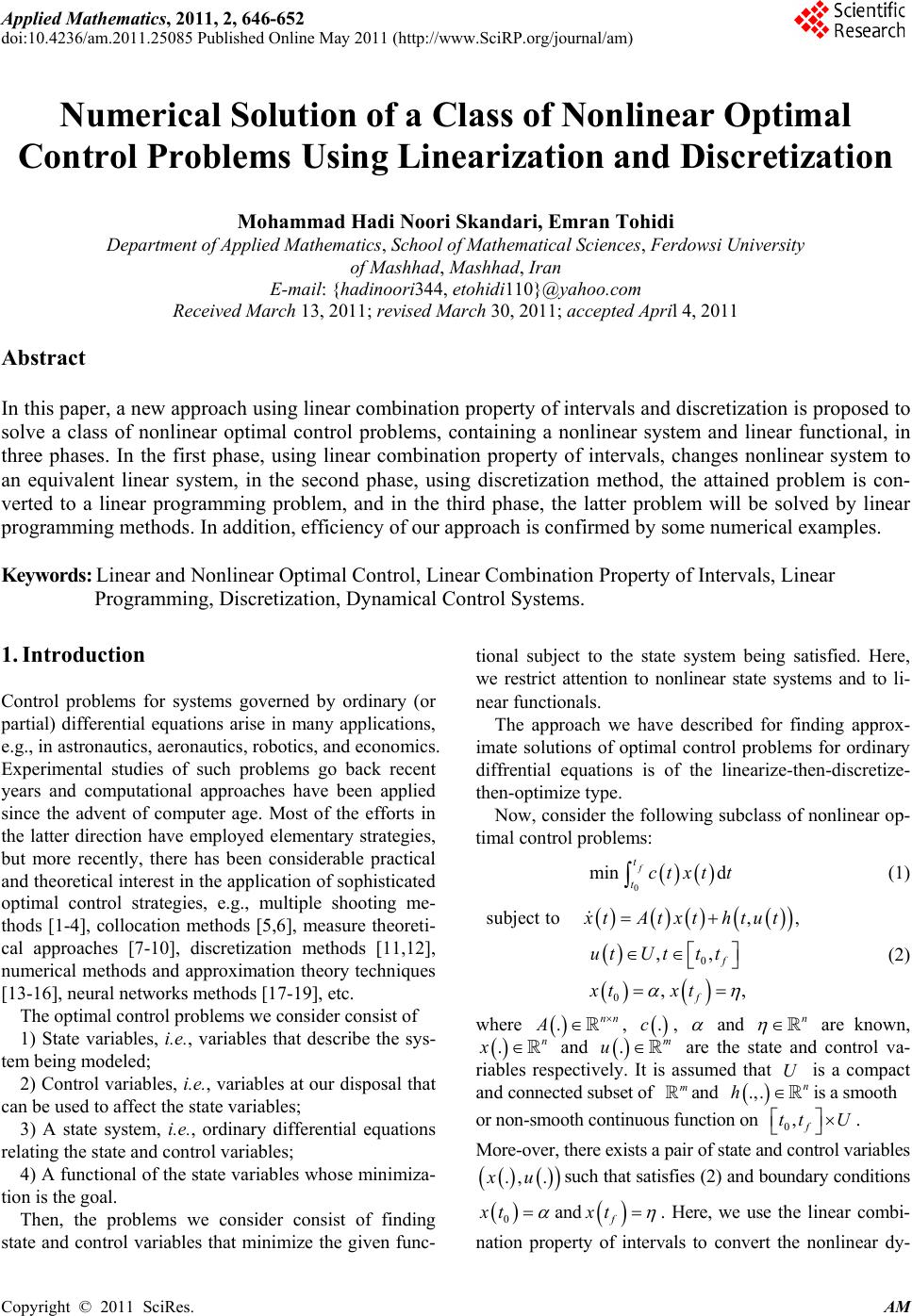
Applied Mathematics, 2011, 2, 646-652
doi:10.4236/am.2011.25085 Published Online May 2011 (http :/ /www.SciRP.org/journal/am)
Numerical Solution of a Class of Nonlinear Optimal
Control Problems Using Linearization and Dis cretization
Mohammad Hadi Noori Skandari, Emran Tohidi
Department of Applied Mathematics, School of Mathematical Sciences, Ferdowsi University
of Mashhad, Mashhad, Iran
Received March 13, 2011; revised March 30, 2011; accepted Ap ril 4, 2011
Abstract
In this paper, a new approach using linear combination property of intervals and discretization is proposed to
solve a class of nonlinear optimal control problems, containing a nonlinear system and linear functional, in
three phases. In the first phase, using linear combination property of intervals, changes nonlinear system to
an equivalent linear system, in the second phase, using discretization method, the attained problem is con-
verted to a linear programming problem, and in the third phase, the latter problem will be solved by linear
programming methods. In addition, efficiency of our approach is confirmed by some numerical examples.
Keywords: Linear and Nonlinear Optimal Control, Linear Combination Property of Intervals, Linear
Programming, Discretization, Dynamical Control Systems.
1. Introduction
Control problems for systems governed by ordinary (or
partial) differential equations arise in many applications,
e.g., in astronautics, aeronau tics, robotics, and economics.
Experimental studies of such problems go back recent
years and computational approaches have been applied
since the advent of computer age. Most of the efforts in
the latter direction have employed elementary strategies,
but more recently, there has been considerable practical
and theoretical interest in the application of sophisticated
optimal control strategies, e.g., multiple shooting me-
thods [1-4], collocation methods [5,6], measure theoreti-
cal approaches [7-10], discretization methods [11,12],
numerical methods and approximation theory techniques
[13-16], neural networks methods [ 17-19], etc.
The optimal control problems we consider consist of
1) State variables, i.e., variables that describe the sys-
tem being modeled;
2) Control variables, i.e., variables at our disposal that
can be used to affect the state variables;
3) A state system, i.e., ordinary differential equations
relating the state and control variables;
4) A functional of the state variables whose minimiza-
tion is the goal.
Then, the problems we consider consist of finding
state and control variables that minimize the given func-
tional subject to the state system being satisfied. Here,
we restrict attention to nonlinear state systems and to li-
near functionals.
The approach we have described for finding approx-
imate solutions of optimal control problems for ordinary
diffrential equations is of the linearize-then-discre tize-
then-optimize type.
Now, consider th e following subclass of nonlinear op-
timal control problems:
( )( )
0
min d
f
t
t
ctxt t
∫
(1)
( )( )( )( ) ( )
( )
( ) ( )
0
0
subject to,,
,,
,,
f
f
xtAtxt htut
utUtt t
xt xt
αη
= +

∈∈

= =

(2)
where
( )
.
nn
A
×
∈
,
( )
.c
,
α
and
n
η ∈
are known,
( )
.
n
x∈
and
( )
.
m
u∈
are the state and control va-
riables respectively. It is assumed that
U
is a compact
and connected subset of
m

and
( )
.,.
n
h∈
is a smooth
or non-smooth continuous func tion on
0
,
f
tt U

×

.
More-over, there exists a pair of state and control variables
( )( )
( )
., .xu
such that satisfies (2) and boundary conditions
( )
0
xt α =
and
( )
f
xt η =
. Here, we use the linear co mbi-
nation property of intervals to convert the nonlinear dy-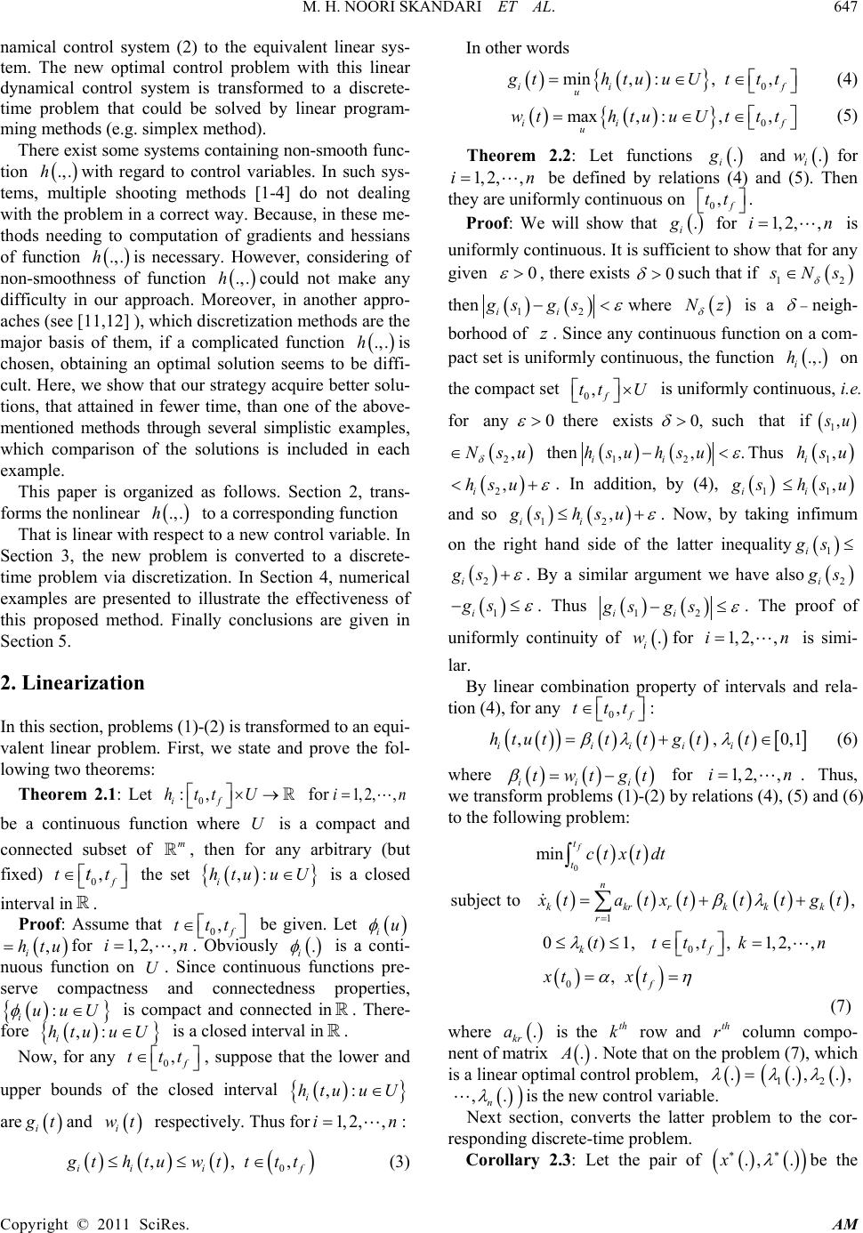

M. H. NOORI SKANDARI ET AL.
647
namical control system (2) to the equivalent linear sys-
tem. The new optimal control problem with this linear
dynamical control system is transformed to a discrete-
time problem that could be solved by linear program-
ming m e t hods (e .g. simplex met hod ) .
There exist some systems containing non-smooth func-
tion
( )
.,.h
with regard to control variables. In such sys-
tems, multiple shooting methods [1-4] do not dealing
with the problem in a correct way. Because, in these me-
thods needing to computation of gradients and hessians
of function
( )
.,.h
is necessary. However, considering of
non-smoothness of function
( )
.,.h
could not make any
difficulty in our approach. Moreover, in another appro-
aches (see [11,12] ), which discretization methods are the
major basis of them, if a complicated function
( )
.,.h
is
chosen, obtaining an optimal solution seems to be diffi-
cult. Here, we show that our strategy acquire better solu-
tions, that attained in fewer time, than one of the above-
mentioned methods through several simplistic examples,
which comparison of the solutions is included in each
example.
This paper is organized as follows. Section 2, trans-
forms the nonlinear
( )
.,.h
to a corresponding function
That is linear with respect to a new control variable. In
Section 3, the new problem is converted to a discrete-
time problem via discretization. In Section 4, numerical
examples are presented to illustrate the effectiveness of
this proposed method. Finally conclusions are given in
Section 5.
2. Linearization
In this section, problems (1)-(2) is transformed to an equi-
valent linear problem. First, we state and prove the fol-
lowing two theorems:
Theorem 2.1: Let
0
:,
if
h ttU

×→
 
for
1, 2,,in=
be a continuous function where
U
is a compact and
connected subset of
m

, then for any arbitrary (but
fixed)
0
,
f
tt t

∈
the set
( )
{ }
,:
i
h tuuU∈
is a closed
interval in

.
Proof: Assume that
0,f
t tt

∈
be given. Let
( )
i
u φ
( )
,
i
h tu=
for
1, 2,,in=
. Obviously
( )
.
i
φ
is a conti-
nuous function on
U
. Since continuous functions pre-
serve compactness and connectedness properties,
( )
{ }
:
i
uuU φ ∈
is compact and connected in

. There-
fore
( )
{ }
,:
i
h tuuU∈
is a closed interval in

.
Now, for any
0
,
f
t tt

∈
, suppose that the lower and
upper bounds of the closed interval
( )
{ }
,:
i
h tuuU∈
are
( )
i
gt
and
( )
i
wt
respec tively. Th us f or
1, 2,,in=
:
( )()( )
( )
0
, ,,
ii if
gth tuw tttt≤≤ ∈
(3)
In other w ords
( )() { }
0
min, :,,
ii f
u
gth tuuUtt t

= ∈∈

(4)
( )() { }
0
max, :,,
ii f
u
w th tuuUttt

= ∈∈

(5)
Theorem 2.2: Let functions
( )
.
i
g
and
( )
.
i
w
for
1, 2,,in=
be defined by relations (4) and (5). Then
they are uniformly co ntinuous on
0,f
tt


.
Proof: We will show that
( )
.
i
g
for
1, 2,,in=
is
uniformly continuous. It is sufficient to show that for any
given
0 ε >
, th ere exists
0 δ >
such that if
( )
12
s Ns
δ
∈
then
( )()
12ii
gs gs ε −<
where
( )
Nz
δ
is a
δ −
neigh-
borhood of
z
. Since any continuous function on a com-
pact set is uniformly continuous, the function
( )
.,.
i
h
on
the compact set
0
,
f
tt U

×

is uniformly continuous, i.e.
for any
0 ε >
there exists
0, δ >
such that if
( )
1,su
( )
2
,N su
δ
∈
then
( ) ()
12
, ,.
ii
hsu hsu ε −<
Thus
( )
1
,
i
hsu
( )
2
,
i
hsu ε <+
. In addition, by (4),
( )
1i
gs
( )
1
,
i
hsu≤
and so
( )()
12
,
ii
gshsu ε ≤+
. Now, by taking infimum
on the right hand side of the latter inequality
( )
1i
gs≤
( )
2i
gs ε +
. By a similar argument we have also
( )
2i
gs
( )
1i
gs ε −≤
. Thus
( )()
12ii
gs gs ε −≤
. The proof of
uniformly continuity of
( )
.
i
w
for
1, 2,,in=
is simi-
lar.
By linear combination property of intervals and rela-
tion (4), for a n y
0
,
f
t tt

∈
:
( )
( )
( )( )( )( )
[ ]
,, 0,1
iiiii
h tutttgtt βλ λ =+∈
(6)
where
( )( )( )
i ii
twt gt β = −
for
1, 2,,in=
. Thus,
we transform problems (1)-(2) by relations (4), (5) and (6)
to the fol l owing pro bl e m:
( )()
( )( )( )( )( )( )
( )
( )
0
1
0
0
min
subject to,
0()1,,,1, 2,,
,
f
t
t
n
kkr rkkk
r
kf
f
ctxtdt
xtatxtttgt
tt ttkn
xt xt
βλ
λ
αη
=
= ++
 ≤ ≤∈=

= =
∫
∑


(7)
where
( )
.
kr
a
is the
th
k
row and
th
r
column compo-
nent of matrix
( )
.A
. Note that on the problem (7), which
is a linear optimal control problem,
( )
. λ =
( )( )
(
12
., ., λλ
( )
)
,.
n
λ 
is the new co ntrol variable.
Next section, converts the latter problem to the cor-
responding discrete-time problem.
Corollary 2.3: Let the pair of
( )( )
( )
., .x λ
∗∗
be t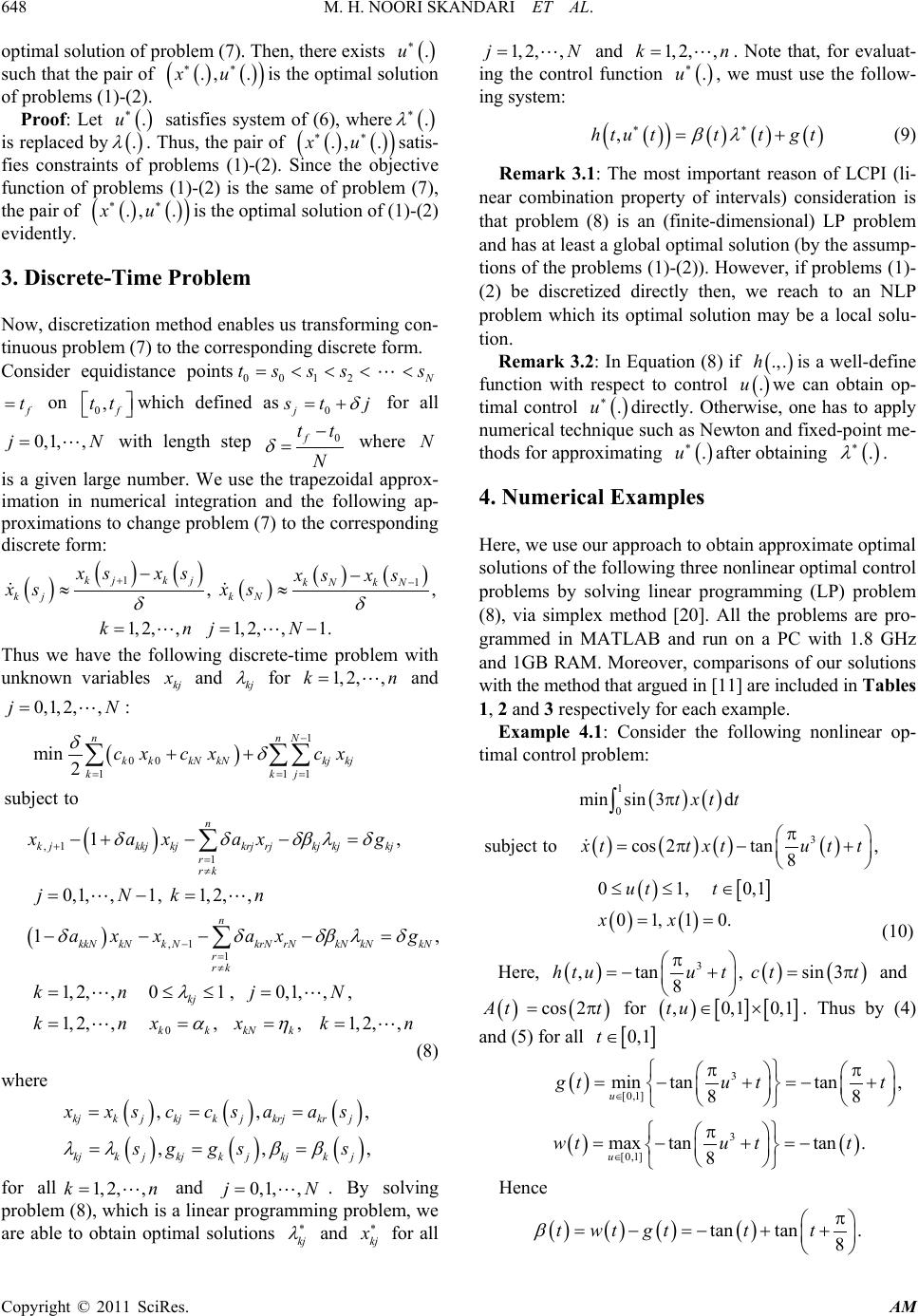he

M. H. NOORI SKANDARI ET AL.
648
optimal solution of problem (7). Then, there exists
( )
.u
∗
such that the pair of
( )()
( )
., .xu
∗∗
is the optimal solution
of problems (1)-(2).
Proof: Let
( )
.u
∗
satisfies system of (6), where
( )
. λ
∗
is replaced by
( )
. λ
. Thus, the pair of
( )()
( )
., .xu
∗∗
satis-
fies constraints of problems (1)-(2). Since the objective
function of problems (1)-(2) is the same of problem (7),
the pair of
( )()
( )
., .xu
∗∗
is the optimal solution of (1)-(2)
evidently.
3. Discrete-Time Problem
Now, discretization method enables us transforming con-
tinuous problem (7) to the corresponding discrete form.
Consider equidistance points
0012
tsss=<<<

N
s<
f
t=
on
0,f
tt


which defined as
0j
st j δ = +
for all
0,1, ,jN=
with length step
0f
tt
N
δ
−
=
where
N
is a given large number. We use the trapezoidal approx-
imation in numerical integration and the following ap-
proximations to change problem (7) to the corresponding
discrete form:
( )()()
( )()()
11
,,
1, 2,,1, 2,,1.
kj kjkN kN
kj kN
xs xsxs xs
xs xs
k nj N
δδ
+−
−−
≈≈
== −


Thus we have the following discrete-time problem with
unknown variables
kj
x
and
kj
λ
for
1, 2,,kn=
and
0,1,2, ,jN=
:
( )
( )
( )
1
00
1 11
,1 1
,1 1
min 2
subject to
1,
0,1, ,1,1,2, ,
1,
1,2, ,01,0,1, , ,
1,
n nN
kkkNkNkj kj
k kj
n
k jkkjkjkrjrjkjkjkj
r
rk
n
kkNkNk NkrNrNkNkNkN
r
rk
kj
c xcxcx
xa xaxg
j Nk n
a xxaxg
kn jN
k
δδ
δδδβλδ
δδδβλδ
λ
−
== =
+=
≠
−=
≠
++
−+−− =
= −=
−−−−=
=≤≤ =
=
∑ ∑∑
∑
∑


0
2, ,,,1,2, ,
kk kNk
nx xk n αη == =
(8)
where
( )( )( )
( )( )( )
,, ,
,,,
kjk jkjk jkrjkrj
kjkjkjk jkjk j
xxsccsaas
s ggss λλ ββ
= ==
= ==
for all
1, 2,,kn=
and
0,1, ,jN=
. By solving
problem (8), which is a linear programming problem, we
are able to obtain optimal solutions
kj
λ
∗
and
kj
x
∗
for all
1, 2,,jN=
and
1, 2,,kn=
. Note that, for evaluat-
ing the control function
( )
.u
∗
, we must use the follow-
ing system:
( )
( )
( )( )( )
,htu tttgt βλ
∗∗
= +
(9)
Remark 3.1: The most important reason of LCPI (li-
near combination property of intervals) consideration is
that problem (8) is an (finite-dimensional) LP problem
and has at least a global optimal solution (by the assump-
tions of the problems (1)-(2)). However , if problems (1)-
(2) be discretized directly then, we reach to an NLP
problem which its optimal solution may be a local solu-
tion.
Remark 3.2: In Equ ation (8) if
( )
.,.h
is a well-define
function with respect to control
( )
.u
we can obtain op-
timal control
( )
.u
∗
directly. Otherwise, one has to apply
numerical technique such as Newton and fixed-point me-
thods for approxi mating
( )
.u
∗
after obta ining
( )
. λ
∗
.
4. Numerical Examples
Here, we use our approach to obtain approximate optimal
solutions of the following three nonlinear optimal control
problems by solving linear programming (LP) problem
(8), via simplex method [20]. All the problems are pro-
grammed in MATLAB and run on a PC with 1.8 GHz
and 1GB RAM. Moreover, comparisons of our solutions
with the method that argued in [11] are included in Tables
1, 2 and 3 respectively for each example.
Example 4.1: Consider the following nonlinear op-
timal control problem:
()()
( )()()( )
( ) [ ]
()( )
1
0
3
minsin 3d
subject tocos2tan,
8
01, 0,1
01, 10.
txt t
xttxtu tt
ut t
xx
π
π

=π− +


≤≤ ∈
= =
∫

(10)
Here,
( )( )()
3
,tan,sin3
8
htuu t ctt
π

=− +=π


and
( )
At
( )
cos 2 t=π
for
( )
[][]
,0,1 0,1tu∈×
. Thus by (4)
and (5) for a ll
[ ]
0,1t∈
( )
3
[0,1]
min tantan,
88
u
gtu tt
∈
π π
 
= −+=−+

 
 

( )( )
3
[0,1]
maxtantan .
8
u
wtu tt
∈
π 

= −+=−




Hence
( )( )( )( )
tan tan.
8
twt gttt β
π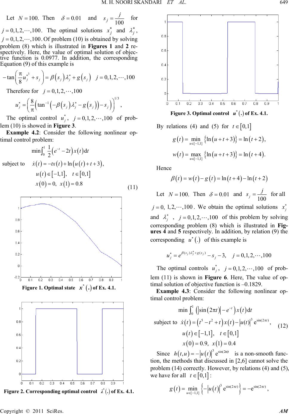

=−=−+ +



M. H. NOORI SKANDARI ET AL.
649
Let
100.N=
Then
0.01 δ =
and
100
j
j
s=
for
0,1,2, ,100.j=
The optimal solutions
j
x
∗
and
j
λ
∗
,
0,1,2, ,100.j=
Of problem (10) is obtained by solving
problem (8) which is illustrated in Figures 1 and 2 re-
spectively. Here, the value of optimal solution of objec-
tive function is 0.0977. In addition, the corresponding
Equation (9) of this example is
( )( )
3
tan0,1,2, ,100
8
j jjjj
u ssgsj βλ
∗∗
π

−+= +=

 
Theref ore for
0,1,2, ,100j=
( )( )
( )
( )
1/3
1
8tan ,
jjjj j
usgs s βλ
∗− ∗

=− −−

π

The optimal control
*
j
u
,
0,1,2, ,100j=
of prob-
lem (10) is showed in F igure 3.
Example 4.2: Consider the following nonlinear op-
timal control problem:
( )
( )
( )()( ) ( )
( ) [][]
()( )
1
0
1
min2 d
2
subject toln3,
1,1,0,1
00,1 0.8
t
etxtt
xttxtut t
ut t
xx
−
−
=− +++
∈− ∈
= =
∫

(11)
Figure 1. Optimal state
( )
*.x
of Ex. 4.1.
Figure 2. Corresponding optimal control
( )
*
.λ
of Ex. 4.1.
Figure 3. Optimal control
( )
*.u
of Ex. 4.1.
By relations (4) and (5) for
[ ]
0,1t∈
( )()
{ }
( )
[ 1,1]
minln3 ln 2,
u
gtu tt
∈−
=++ =+
( )()
{ }
( )
[ 1,1]
maxln3ln 4.
u
wtu tt
∈−
=++=+
Hence
( )( )( )() ()
ln 4ln 2twt gttt β =−=+− +
Let
100.N=
Then
0.01 δ =
and
100
j
j
s=
for all
0,j=
1,2, ,100
. We obtain the optimal solutions
j
x
∗
and
j
λ
∗
,
0,1,2, ,100j=
of this problem by solving
corresponding problem (8) which is illustrated in Fig-
ures 4 and 5 respectively. In addition, by relation (9) the
corresponding
( )
.u
∗
of this example is
() ()
3,0,1,2, ,100
jj j
s gs
jj
ues j
βλ
∗
+
∗
=−− = 
The optimal controls
*
j
u
,
0,1,2, ,100j=
of prob-
lem (11) is shown in Figure 6. Here, The value of op-
timal solution of objective function is –0.1829.
Example 4.3: Consider the following nonlinear op-
timal control problem:
( )
( )
( )
( )
( )
( )
( ) [][ ]
()( )
1
0
3
52sin(2 )
minsin 2d
subject to()e,
1,1 ,0,1
00.9,10.4
t
t
text t
xtt ttxtut
ut t
xx
−
π
π−
= −+−
∈− ∈
= =
∫

(12)
Since
()( )
3sin(2π)
,e
t
htu ut= −
is a non-smooth func-
tion, the methods that discussed in [2,6] cannot solve the
problem (14) correctly. However, by relations (4) and (5),
we have for all
[ ]
0,1t∈
:
( )( )
{ }
3sin(2 )sin(2 )
[ 1,1]
minee,
tt
u
gt ut
ππ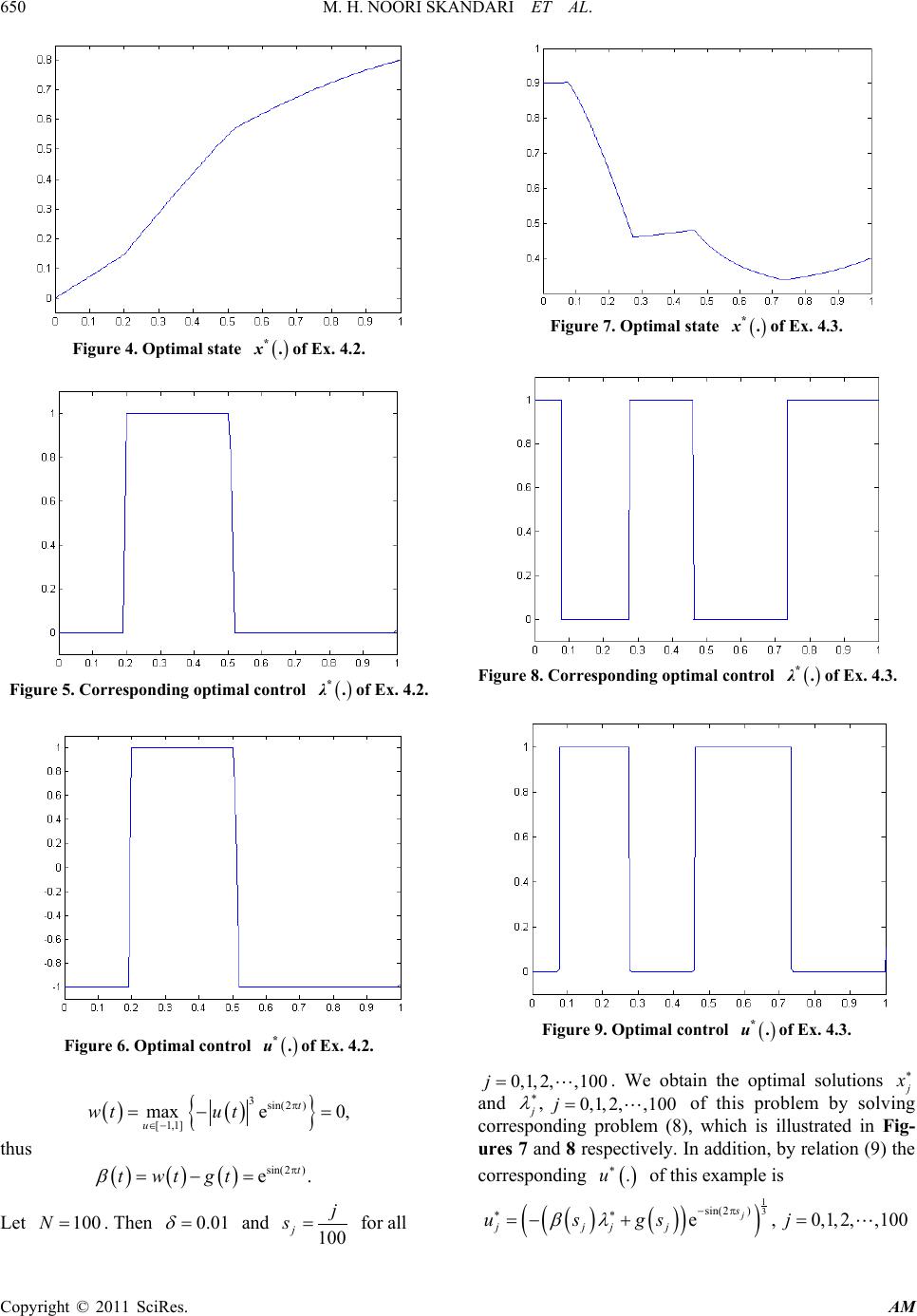
∈−
=−=−

M. H. NOORI SKANDARI ET AL.
650
Figure 4. Optimal state
( )
*
.x
of Ex. 4.2.
Figure 5. Corresponding optimal control
( )
*.λ
of Ex. 4.2.
Figure 6. Optimal control
( )
*.u
of Ex. 4.2.
( )()
{ }
3sin(2 )
[ 1,1]
maxe 0,
t
u
wt ut
π
∈−
=−=
thus
( )( )( )
sin(2 )
e.
t
twtgt β
π
=−=
Let
100N=
. Then
0.01 δ =
and
100
j
j
s=
for all
Figure 7. Optimal state
( )
*
.x
of Ex. 4.3.
Figure 8. Corresponding optimal control
( )
*.λ
of Ex. 4.3.
Figure 9. Optimal control
( )
*
.u
of Ex. 4.3.
0,1,2, ,100j=
. We obtain the optimal solutions
j
x∗
and
,
j
λ
∗
0,1,2, ,100j=
of this problem by solving
corresponding problem (8), which is illustrated in Fig-
ures 7 and 8 respectively. In addition, by relation (9) the
corresponding
( )
.u
∗
of this example is
( )()
( )
( )
1
3 sin(2 )
e,0,1,2, ,100
j
s
jjjj
usgsj βλ
−π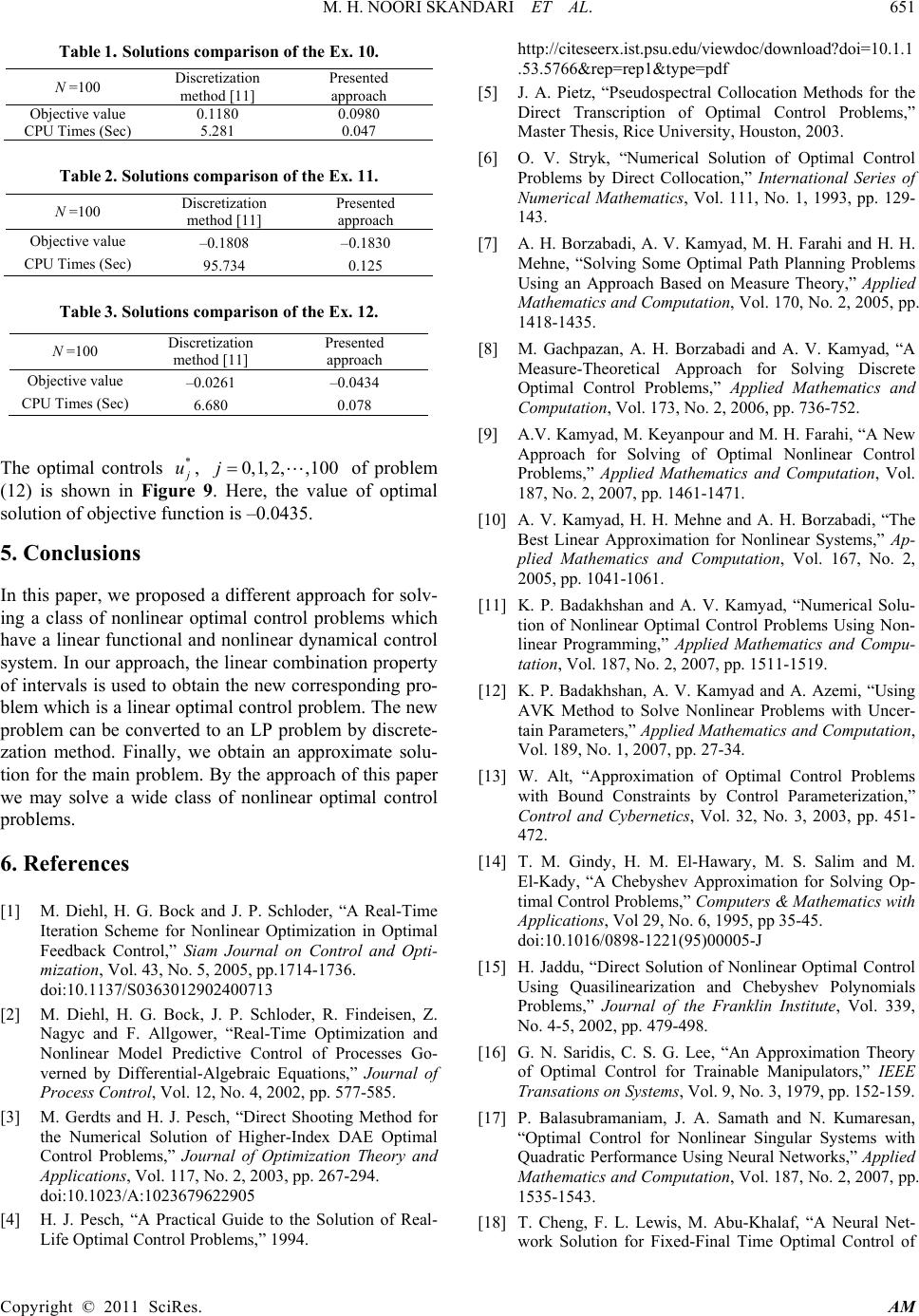
∗∗
=−+ =

M. H. NOORI SKANDARI ET AL.
651
Table 1. Solutions comparison of the Ex. 10.
N =100
Discretization
method [11]
Presented
approach
Objective value
0.1180
0.0980
CPU Times (Sec)
5.281
0.047
Table 2. Solutions comparison of the Ex. 11.
N =100
Discretization method [11]
Presented approach
Objective value –0.1808 –0.1830
CPU Times (Sec) 95.734 0.125
Table 3. Solutions comparison of the Ex. 12.
N =100 Discretization method [11] Presented ap p ro ach
Objective value –0.0261 –0.0434
CPU Times (Sec)
6.680 0.078
The optimal controls
*
j
u
,
0,1,2, ,100j=
of problem
(12) is shown in Figure 9. Here, the value of optimal
solution of objective function is –0.0435.
5. Conclusions
In this paper, we proposed a different approach for solv-
ing a class of nonlinear optimal control problems which
have a linear functional and nonlinear dynamical control
system. In our approach, the linear combination property
of intervals is used to obtain the new corresponding pro-
ble m wh ich is a linear optimal control problem. The new
problem can be converted to an LP problem by discrete-
zation method. Finally, we obtain an approximate solu-
tion for the main problem. By the approach of this paper
we may solve a wide class of nonlinear optimal control
problems.
6. References
[1] M. Diehl, H. G. Bock and J. P. Schloder, “A Real-Time
Iteration Scheme for Nonlinear Optimization in Optimal
Feedback Control,” Siam Journal on Control and Opti-
mization, Vol. 43, No. 5, 2005, pp.1714-1736.
doi:10.1137/S0363012902400713
[2] M. Diehl, H. G. Bock, J. P. Schloder, R. Findeisen, Z.
Nagy c and F. Allgower, “Real-Time Optimization and
Nonlinear Model Predictive Control of Processes Go-
verned by Differential-Algebraic Equations,” Journal of
Process Control, Vol. 12, No. 4, 2002, pp. 577-585.
[3] M. Gerdts and H. J. Pesch, “Direct Shooting Method for
the Numerical Solution of Higher-Index DAE Optimal
Control Problems,” Journal of Optimization Theory and
Applications, Vol. 117, No. 2, 2003, pp. 267-294.
doi:10.1023/A:1023679622905
[4] H. J. Pesch, “A Practical Guide to the Solution of Real-
Life Optimal Control Problems,” 1994.
http://citeseerx.ist.psu.edu/viewdoc/download?doi=10.1.1
.53.5766&rep=rep1&type=pdf
[5] J. A. Pietz, “Pseudospectral Collocation Methods for the
Direct Transcription of Optimal Control Problems,”
Master Thesis, Ric e University, Houston, 2003.
[6] O. V. Stryk, “Numerical Solution of Optimal Control
Problems by Direct Collocation,” International Series of
Numerical Mathematics, Vol. 111, No. 1, 1993, pp. 129-
143.
[7] A. H. Borzabadi, A. V. Kamyad, M. H. Farahi and H. H.
Mehne, “Solving Some Optimal Path Planning Problems
Using an Approach Based on Measure Theory,” Applied
Mathematics and Computation, Vol. 170, N o. 2, 2005, pp.
1418-1435.
[8] M. Gachpazan, A. H. Borzabadi and A. V. Kamyad, “A
Measure-Theoretical Approach for Solving Discrete
Optimal Control Problems,” Applied Mathematics and
Computation, Vol. 173, No. 2, 2006, pp. 736-752.
[9] A.V. Kamyad, M. Keyanpour and M. H. Farahi, “A New
Approach for Solving of Optimal Nonlinear Control
Problems,” Applied Mathematics and Computation, Vol.
187, No. 2, 2007, pp. 1461-1471.
[10] A. V. Kamyad, H. H. Mehne and A. H. Borzabadi, “The
Best Linear Approximation for Nonlinear Systems,” Ap-
plied Mathematics and Computation, Vol. 167, No. 2,
2005, pp. 1041-1061.
[11] K. P. Badakhshan and A. V. Kamyad, “Numerical Solu-
tion of Nonlinear Optimal Control Problems Using Non-
linear Programming,” Applied Mathematics and Compu-
tation, Vol. 187, No. 2, 2007, pp. 1511-1519.
[12] K. P. Badakhshan, A. V. Kamyad and A. Azemi, “Using
AVK Method to Solve Nonlinear Problems with Uncer-
tain Parameters,” Applied Mathematics and Computation,
Vol. 189, No. 1, 2007, pp. 27-34.
[13] W. Alt, “Approximation of Optimal Control Problems
with Bound Constraints by Control Parameterization,”
Control and Cybernetics, Vol. 32, No. 3, 2003, pp. 451-
472.
[14] T. M. Gindy, H. M. El-Hawary, M. S. Salim and M.
El-Kady, “A Chebyshev Approximation for Solving Op-
timal Control Problems,” Computers & Mathematics with
Applications, Vol 29, No. 6, 1995, pp 35-45.
doi:10.1016/0898-1221(95)00005-J
[15] H. Jaddu, “Direct Solution of Nonlinear Optimal Control
Using Quasilinearization and Chebyshev Polynomials
Problems,” Journal of the Franklin Institute, Vol. 339,
No. 4-5, 2002, pp. 479-498.
[16] G. N. Saridis, C. S. G. Lee, “An Approximation Theory
of Optimal Control for Trainable Manipulators,” IEEE
Transations on Systems, Vol. 9, No. 3, 1979, pp. 152-159.
[17] P. Balasubramaniam, J. A. Samath and N. Kumaresan,
“Optimal Control for Nonlinear Singular Systems with
Quadratic Performance Using Neural Networks,” Applied
Mathematics and Computation, Vol. 187, No. 2, 2007, pp.
1535-1543.
[18] T. Cheng, F. L. Lewis, M. Abu-Khalaf, “A Neural Net-
work Solution for Fixed-Final Time Optimal Control of

M. H. NOORI SKANDARI ET AL.
652
Nonlinear Systems,” Automatica, Vol. 43, No. 3, 2007,
pp. 482-490.
[19] P. V. Medagam and F. Pourboghrat, “Optimal Control of
Nonlinear Systems Using RBF Neural Network and
Adaptive Extended Kalman Filter,” Proceedings of
American Control Conference Hyatt Regency Riverfront,
St. Louis, 10-12 June 2009, pp. 355-360.
[20] D. Luenberger, “Linear and Nonlinear Programming,”
Kluwer Academic Publishers, Norwell, 1984.