Applied Mathematics, 2011, 2, 586-594
doi:10.4236/am.2011.25078 Published Online May 2011 (http://www.SciRP.org/journal/am)
Influence of Rigid Boundary and Initial Stress on the
Propagation of Love Wave
Shishir Gupta, Amares Chattopadhyay, Sumit K. Vishwakarma, Dinesh K. Majhi
Department of Ap pl ie d M athematics, Indian School of Mines, Dhanbad, India
Received March 10, 2011; revised March 24, 2011; accepted March 28, 2011
Abstract
In the present paper we study the effect of rigid boundary on the propagation of Love waves in an inhomo-
geneous substratum over an initially stressed half space, where the heterogeneity is both in rigidity and den-
sity. The dispersion equation of the phase velocity has been derived. It has been found that the phase velocity
of Love wave is considerably influenced by the rigid boundary, inhomogeneity and the initial stress present
in the half space. The velocity of Love waves have been calculated numerically as a function of KH (where
K is a wave number H is a thickness of the layer) and are presented in a number of graphs.
Keywords: Love Waves, Initial Stress, Heterogeneous Half-Space, Rigid Boundary, Phase Velocity
1. Introduction
The earth is a non-homogeneous medium with variations
in density and rigidity in constituent layer. A study on
earth structure and earth quakes [1,2] says that inside the
earth there exist materials which are anisotropic in nature
i.e., deviate from the directionally regular elastic behav-
iour of an isotropic material. The study of generation and
propagation of waves in layered anisotropic media, with
various geometrical configurations are important in
Geophysics, Seismology, Acoustic and Electromagnet-
ism. Theoretical studies of anisotropy usually dealt with
limiting case such as infinitesimal thickness and infinite
wavelength, or with infinite thickness and infinite fre-
quency. According to some seismologists anisotropy is
the limiting case of a laminated solid as the laminations
become infinitesimal, and Stoneley considers surface
wave propagation along a half space.
The effect of inhomogeneity and rigid boundary on
Love wave propagation is becoming increasingly impor-
tant as seismologists study the structure of earth in ever
finer details. Love waves are more sensitive to structural
complexities than are Rayleigh waves. The propagation
of Love waves in a medium having different types of
crustal thickness was discussed by Satô [3] and De Noy-
er [4].
Propagation of Love waves under some particular
physical conditions which are likely to exist in the inte-
rior of the earth is studied in this paper. It is Love [5],
who first predicted that the earth is in a state of high ini-
tial stress. Due to atmospheric pressure, gravity vibration,
creep, difference in temperature, large initial stresses
may exist inside the earth. The stresses which exist in an
elastic body even though external forces are absent are
termed as initial stresses and the body is said to be ini-
tially stressed. These stresses might exert significant in-
fluence on the elastic waves produced by earthquakes,
explorations or impacts. Thus, it is imperative to deal
with the properties of wave propagation under initial
stress. It was Biot [6] who first pointed out that the initial
stress influences elastic waves to a great extent. The the-
ory of incremental deformation formulated by Biot [7] in
his famous book “Mechanics of Incremental Deforma-
tion” has been employed by several authors to study the
propagation of surface waves in pre-stressed elastic sol-
ids. Propagation of Love waves in a non-homogeneous
orthotropic elastic layer under initial stress overlying
semi-infinite medium is studied by Abd-Alla and Ahmed
[8]. Khurana [9] has shown the effect of initial stress on
the propagation of Love wave. Wave velocities in a
pre-stressed anisotropic elastic medium have been stud-
ied by Sharma and Garg [10]. References to be made to
Das and Dey [11,12], Dey [13], Dey and Addy [14],
Chattopadhyay and De [15], Chattopadhyay and Kar [16]
and others. They suggested that the studies on the prob-
lem of elastic wave inside the earth deserve the consid-
eration of initial stresses present in the medium. These
stresses might exert significant influence on the elastic

S. GUPTA ET AL.587
waves produced by earthquakes, explorations or impacts.
Thus, it is imperative to deal with the problems of wave
propagation under initial stress.
The near surface of the earth consists of layers of dif-
ferent types of material properties overlying a half space
of various types of rock, underground water, oil & gases.
So, the studies of the propagation of seismic waves will
be of great interest to seismologist. A detail study on
elastic wave propagation and its generation in seismol-
ogy had been made by Pujol [17] and Chapman [18]. In
the present paper Love wave propagation in anisotropic
layer of sandstone with rigid boundary over a pre-
stressed orthotropic quartz medium has been studied.
The inhomogeneity of the layer is taken into considera-
tion by assuming
 
22
00
1, 1
N
NmzLLmz 
2
and , m is a constant and having dimen-

01mz
 


sion that is inverse of length. Also the inhomogeneity of
the half-space has been taken as

11az

 and

11bz


 where a, b are constants and having di-
mensions that are inverse of length. The initial stresses P
present in the inhomogeneous quartz half space also have
effect in the velocity of propagation. The initial com-
pressive stress is seen to reduce the velocity. The upper
boundary plane of the layer is assumed to be rigid, and
both the rigidity and the mass density of the underlying
half space are assumed to increase linearly with depth.
2. Formulation and Solution of the Problem
Consider an inhomogeneous anisotropic layer of finite
thickness
H
over an initially stressed inhomogeneous
quartz half-space. We assume that the upper surface of
the crustal layer is rigid and horizontal. The -axis is
taken vertically downwards in the lower medium. The
z
x
-axis is chosen parallel to the layer in the direction of
wave propagation, origin being taken at the depth
H
below the upper surface of the layer as shown in Fig-
ure 1. and
,NL

are the directional rigidities and
density at any point in the layer which is assumed to be
transversely isotropic with z-axis as the axis of sym-
metry. The inhomogeneity of the layer has been taken as
 
22
00
1, 1NNmz LLmz 
and

2
01mz

 ,
mis a constant and having dimension that is inverse of
length. In the half space rigidity and density vary linearly
with depth i.e.


11az
  and
where are constants and having dimensions that are
inverses of length.

11bz
 
,ab
2.1. Solution for the Layer
Let and be the displacement components in
the x, y and z direction respectively. Starting from the
general equation of motion and using the conventional
Love waves conditions viz., and
,uv w
0, 0uw


1,,vvxzt, the only y component. Then the equation
of motion in absence of body force can be written as [7]
22
11
22
vv
NL
zz
1
v
x
t


 





 (1)
For a wave propagating along
x
-direction, we may
assume


1eiK xct
vVz  

(2)
Using Equation (2), Equation (1) takes the form

22
2
2
d1dd 0
dd d
VLVK
cNV
Lz zL z


 (3)
After putting 1
V
VL  in Equation (3), we get
Figure 1. Geometry of the problem.
P



1
1
1
1
az
bz







2
0
2
0
2
0
1
1
1
N
Nmz
LL mz
mz 



H Inhomogeneous Anisotropic
Layer
Inhomogeneous Quartz
Half-Space
Z = 0
Z = –H
Rigid boundary
x
P
z

S. GUPTA ET AL. 588

2
222
2 1
11
222
d1d1 d0
2d dd4
VLLK
VVcN
LzL zzL


 

 1
V


(4)
The variations in rigidities and density are taken as
 
22
00
1, 1NNmzLLmz 
and

2
01mz
 
(5)
wheremis a constant having dimension inverse of leng-
th.
Using Equation (5), Equation (4) changes to
2
2 1
11
2
d0
d
VmV
z (6)
where

2
22
10
0
K
mcN
L
 

0
(7)
The solution of Equation (6) may be assumed as
11
1ee
im zim z
VA B


Thus the solution for the non-homogeneous, anisot-
ropic layer may be taken as


11
1
0
e
ee
1
im zim ziK xct
AB
vLmz




(8)
2.2. Solution for the Half-Space
The lower medium is considered as inhomogeneous
quartz half-space under initial horizontal compressive
stress along x-axis. The eqn. of motion correspond-
ing to the displacement due to Love waves can be written
as [7]
P

22
23 21
2
22
2
s sPv v
xz xt


 
 

 


(9)
whereij
s
are the incremental stress components in the
half-space, is the initial compressive stress along the
x-direction, and
P

is the density of the material of the
half space. In the present problem we have


11az
 and 1

 

1bz

(10)
Using the stress-strain relations
21 23
2, 2
x
yyz
s
es e


 (11)
And the relation (10), the equation of motion (9) can
be written as



22 2
1
22 2
22
11
1
1211 1
bz
vv vv
Pa
azaz zaz
2
2
x
zt


 
 






 (12)
Let


2e
x
ctiK
vVz  (13)
be the solution of Equation (12).
Using Equation (13), Equation (12) takes the form

 
2
12
2
11
1
dd 1
1d 121 d
bz
VaV P
c
az zazaz
z



 
 


 
 


2
0K V 

(14)
Putting


1/2
()
1
z
Vaz


in Equation (14) to eliminate the term dV
dz , we get
 



22
// 2
22
1
1
() 10
21 1
41 os
bz
aPc
zK
az az c
az






z


  












(15)
where 1
0
os
c


and is phase velocity. Substituting c


1/ 2
2
1
12
1
21
1, ,
21 os
Kaz
Pcb
K
c
az aa c





 





in Equation (15) we get

2
22
d11
0
24 d4
R 
 

 


(16)
where


2
22
1os
ab
RcaK



Equation (16) is a Whittaker’s
equation, solution of which may be written as

S. GUPTA ET AL.589
  
12,02 2,0RR
DW DW



  
where 1 and 2 are arbitrary constants and
/2,0R
D

D
W

is the Whittaker’s function. The solution of
Equation (16) satisfying the condition when
i.e.
lim z

Vz0lim

 when may be ta-
ken as

0  
 
1/2,0R
DW

   (17)
Hence, the displacement component in the heteroge-
neous half-space is given by





12,0
2ee
112
R iKxctikx ct
DW
vVz az





(18)
Expanding Whittaker’s function up to linear terms
Equation (18) reduces to

 

1
21
2
/2
(1 )
1
1/ 23/ 2
1
1
21 2
1
ee
121
KR
az iK xct
a
K
Ra
az
vD aaz az


 





 







 







(19)
Boundary Conditions and Dispersion equation




12
1
At the interface, 0 the continuity of the stress requires that
At rigid boundary , the displacement is vanishing so that =0, at
and the continuity of the displacement requires
yz y
zf
zHv zH
 
 
12
that at 0 vv z







(20)
where
y
f
 is the incremental boundary force per unit
initial area in the pre-stressed half-space at deformed
stage, the physical explanations of which may be ob-
tained from Figure 2. In the boundary conditions the
quantities (i.e.
y
f
and for the stratum (inhomoge-
neous and anisotropic) and lower half-space are denoted
by the subscripts 1 and 2 respectively.
)v
The magnitude of
y
f
as derived by [7] is

iij ij kjikik jk

j
f
sSwSeSen 
where are the initial stress components,
ij
Sij
s
are the
incremental stress components, are the strain com-
ponents, are the rotational components, is the
dilatation and
ij
e
ij
we
j
nis the cosine of angle between the th
j
direction and normal to the surface. It is obvious that
z
f

is the incremental normal force per unit area to the
boundary whereas,
x
f

and
y
f
are shear forces. In the
present problem, since is the only initial stress com-
11
S
ponent,


,,xzt
222 2
0vv w,u0,

 and also z- axis
is normal to the boundary.
2
23yv
fs z 


Using boundary conditions (20) in Equation (8) and
Equation (19), we get




01001011 0AL immLBL immLDK


0
(21)
11
ee
im HimH
AB


 (22)
102
0AB DLK

 (23)
where
1
1
22
/2
1
10 1
11
2
/2
1
2
1
11
2322
e1
2222 2
1
22
e1
2
R
K
a
R
K
a
RR
aa
aa aR
KK
aKK
Ra
KaK
















 
.,






 
 
  










 








Eliminating ,
A
Band from Equations (21)-(23), we get
1
D


01 001 01
11
e e 0
1
im Him H
LimmLLimmLK

 
02
0
1 LK  

S. GUPTA ET AL. 590
(a) (b) (c)
Figure 2. Incremental bounda r y forc es.
Expanding the above determinant and solving, we get
z
∆fz
∆fx
∆fy
x
y
z
= 0
p
2
00 102
0021
m
(24) cot cN KH LLK






KLKm


Putting the values of 12 ,
K
Kand 1 min Equation (24),
we get
2N01
2
02 0
otcc

A
KH LA
c





(25)
where
222
2
1 1
3 22 aa
01
111
111
2
11
222222
RRR
aa
aR
A
Lm 


 

 

K
KKK



 
 
  


 


 
 
 



 


 


 



2
2
00
20
01
1
2
12
Ra
cN
ALK LK














1/2
2
0
01 2
0
, 1.
os
Lcb
ca
c






and
1
2
P



itial stress P
is the
non-dimensional parameter due to in
The Equation (25) gives the phase velocity of Love
in an inhomogeneous anisotropic layer over an
initially stressed inhomogeneousspace wh
upper boundary plane of the layer is assumed to be rigid.
3.
If the half-space is taken as Gibson half-space i.e., ri-
gidity varies linearly with depth whereas the density re-
mains constant. In this case but so that
.
wave
half en the
Particular Cases
Case 1
0a0b
1



the form
(constant) and the disp Equ25) takes ersionation (
2
01
2
02 0
cot N
A
c
KH LA
c

 


(26)
where

2
11RR
22
2
1 1
111
1
3 222
11
222 22
R
aa
aa aR
10 2
A
L




 




m K
KKK



 
 

 


 


 
 
 



 


 


 



2
2
00
20
01
1
2
12
Ra
cN
ALK LK















S. GUPTA ET AL.591

1/2
11
  ,
2
2
1os
RcaK



which is the dispersion equation of Love wave in an in-
homogeneous layer lying over an initially stressed Gib-
son half space, when the upper boundary plane of the
layer is assumed to be rigid
Case 2
If 0, 0, 0, 0apbmthen the dispersion Equ-
ation (25) takes the form
2
01
2
0
cot N
02
A
c
KH c

 


LA


where
2
10
1
22
2
11
11
1Ra
2
12
11
322
1
22 22 2
AL mK
RR
a
aa aR
K
KK






 



 


 


 


 

 
















2
2
00
20
01
1
2
12
Ra
cN
ALK LK














which is the dispersion equation of Love wave in a ho-
mogeneous layer over an initially stressed half space
with constant density and when upper boundary plane is
assumed to be rigid.
Case 3
If 0, 0, 0abP and 0mthen the dis-
persion Equation (25) takes the form
2
01
cot NA
c
KH




2
02
0LA
c

where 11 AK

 and


2
00
0
2
N
ALK
 

0
c
L
which is the dispersion equation of Loveave in a ho-
mogeneous layer over a homogeneous half-space, when
the upper boundary plane is assumed to be rigid and half-
free from initial stress.
4
w
space is
Case
If 0, 0, 0abP and 0m and
00
NLthen the dispersion Equation (25) takes the form
2
21c
L
c

2
22
0
tan 1o
o
c
KH cc
2
11
os
c



 (27)
Equation (27) gives the phase velocity of Love wave
in a homogeneous isotropic layer over a homogeneous
half space when the upper boundary plane of the layer is
assumed to be rigid and half space has no initial stress.
Note that the equation for the phase velocity c of the
Love waves in a layer overlaying a half-space, when the
upper boundary plane is not rigid, is given by
 
2
12
21
22
0
021
o
c
Lc


It can be seen from Equation (27) and Equation (28)
that the phase velocity of Love waves in a layer with
1
tan 1
c
c
c
KH c





 (28)
a
rig
4. Numerical Computation and Discussion
In order to show the effect of rigid boun
non-homogeneity and initial stresses on
of Love waves, numerical computation of Equation (25)
were performed with different values of parameter (Ta-
bl
id surface is different from that in a layer with a free
surface.
dary, anisotropy,
the propagation
e 1) representing the above characteristics. The value of
os
cc and mKare taken as 0.7 and 0.2 respectively in
all the figure except Figures 9 and 10. In Figures 3-5
curves are plotted when both density as well as rigidity
varies linearly with depth in presence of rigid boundary
ted
when rigidity varies linearly with depth but density
under ffect
plane. Unlike to this, Figures 6-8 have been plot
re-
mains constant, thus giving dispersion curve in Gibson
half space.
Figures 3 and 6 gives the dispersion curves in the ab-
sence of initial stress, shows that the velocity of Love
wave decreases rapidly when the values of KH increases
the e of rigid boundary and initial stress. This
also reflects that the velocity of Love wave is finite in the
vicinity of the surface of the half-space and vanishes as
depth increases for a particular wave number. Moreover,
in the presence of rigid boundary, it has been found that
the velocity of Love wave increases for a particular value
of KH when compared with the case of a layer having
free surface.
Figures 4 and 5 show the effect of initial stress pre-
sent in the half-space. It has been observed that an in-
crease in compressive initial stresses

0  deceases
the velocity of Love waves for the same frequency. The
tensile initial stress


0 

of small magnitude in the
half-space increase the velocity, but the large magnitude
of tensile stress

doesn’t allow Love wave to propagate.
Figures 6 and 7 show the influence of tensile initial
stress in Gibson half-space.
Figure 9 gives the velocity of Love waves for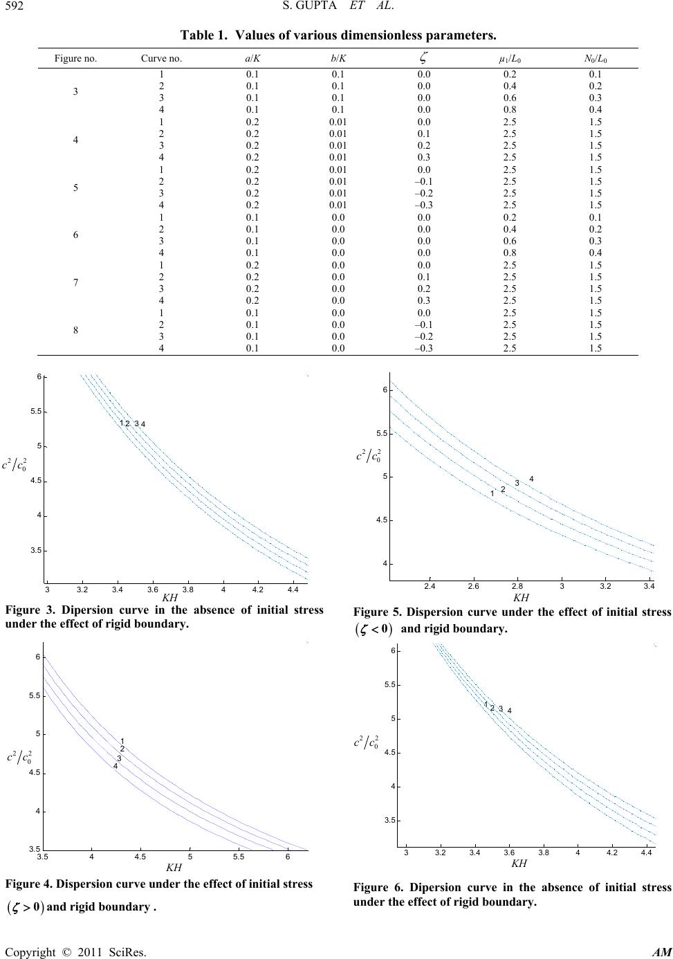

S. GUPTA ET AL. 592
3.5 44.5 55.5 6
3.5
4
4.5
5
5.5
6
KH
0 2
1
c
2
/c
2
3
4
diters.
no. Curve no. a/K b/K
Table 1. Values of various
Figure
mensionless parame

µ1/L0 N0/L0
3
1
2
3
4
0.1
0.1
0.1
0.1
0.0
0.0
0.0
0.0
0.2
0.4
0.6
0.
0.1
0.2
0.3
0.1
0.1
0.1
0.1 8 0.4
4 3
01
0.3
2.5 1.5
1
2
0.2 0.
4
0.2
0.2
0.01
0.01
0.1
0.2
0.2 0.01
0.0 2.5
2.5
1.5
1.5
2.5 1.5
5
1
2
3
4
1
0.2
0.2
0.2
0.2
0.1
0.01
0.01
0.01
0.01
0.0
0.0
–0.1
–0.2
–0.3
0.0
2.5
2.5
2.5
2.5
0.2
1.5
1.5
1.5
1.5
0.1
6 2
3
4
0.1
0.1
0.1
0.0
0.0
0.0
0.0
0.0
0.0
0.4
0.6
0.8
0.2
0.3
0.4
7
1
2
3
4
1
0.2
0.2
0.2
0.2
0.1
0.0
0.0
0.0
0.0
0.0
0.0
0.1
0.2
0.3
0.0
2.5
2.5
2.5
2.5
2.5
1.5
1.5
1.5
1.5
1.5
8 2
3
4
0.1
0.1
0.1
0.0
0.0
0.0
–0.1
–0.2
–0.3
2.5
2.5
2.5
1.5
1.5
1.5
igure 3. Dipersion curve in the absence of initial stress
nder the effect of rigid boundary.
Figure 4. Dispersion curve under the effect of initial stress
and rigid boundary .
F
u


0  
Figure 5. Dispersion curve under the effect of initial stress


0 

and rigid boundary.
igure 6. Dipersion curve in the absence of initial F stress
nder the effe ct of rigid boundary. u
33.2 3.4 3.6 3.8 44.2 4. 4
3. 5
4
4. 5
5
5. 5
6
KH
c
1
2 2
/c
0
23 4
2.4 2.6 2.8 33.2 3.4
4
4. 5
5
5. 5
6
KH
c
2
/c
0 2
1234
33.2 3.4 3.6 3.844.2 4.4
3.5
4
4.5
5
5.5
6
KH
1
c
2
/c
0 2
234
KH
KH
KH
KH
22
c0 c
22
0
cc
22
0
cc
22
0
cc

S. GUPTA ET AL.593
igure 7. Dispersion curve under the effect of initial stress F


0  and rigid boundary .
ress Figure 8. Dispersion curve under the effect of initial st


0  and rigid boundary.
Figure 9. Dimensionless phase speed 22
0
cc as function of
imensionless KH evaluated from Equation (27) for d
.,.,.
0110 1520
 Land

2.
0os02cc .
5
Figure 10. Dimensi onless phas e spee d 22
0
cc as function of
dimensionless KH evaluated from Equation (28) for
.,.,.
0110 1520
 L and

2.
0os02cc .

2
01 0.2cc  in a layer overmogeneous half-space
e la
a ho
when the upper boundary plane of thyer is assumed
to be rigid. While Figure 10 gives the speed of Love
waves for

2
cc ous layer over a
01 .2in a homog
r
r
ckwell
Publishing, Ox003.
] P. M. Shearer, “Introduction to Seismology,” 2nd Edition,
Cambridge
yo, Tokyo, 1952
Publication, New York,
0ene
homogeneous half-space in the absence of rigid bound-
y plane. It is observed that overburden layer has a
rominent effect. It is also observed that magnitudes of
peed are changed in entire range of KH along with re-
ersing the positions of the curve.
ledgements
he author conveys their sincere thanks to Indian School
f Mines, Dhanbad, for providing JRF, Mr. Sumit Kuma
ishwakarma and also facilitating us with best facility.
e are also grateful to the honourable referees for their
valuable suggestions for improving the manuscript.
. References
a
p
s
v
5. Acknow
T
o
V
W
in
6
[1] S. Stein and M. Wysession, “An Introduction to Seis-
mology, Earthquakes and Earth Structure,” Bla
ford, 2
[2
University Press, Cambridge, 2009.
[3] Y. Satô, “Study on Surface Waves VI: Generation of
Love and Other Type of SH-Waves,” Departmental Bul-
letin Paper, Bulletin Earthquake Research Institute, Uni-
versity of Tok, pp.101-120.
[4] J. D. Noyer, “The Effect of Variations in Layer Thickness
on Love Waves,” Bulletin of Seismology Society of Ame-
rica, Vol. 51, No. 2, 1961, pp. 227-235.
[5] A. E. H. Love, “A Treatise on Mathematical Theory of
Elasticity,” 4th Edition, Dover
22.2 2.4 2.62.833.2
4
4.5
5
5.5
6
KH
1 c
2
/c
0 2
2
3
4
22.22.42.62.833.2
3.5
4
4.5
5
5.5
6
KH
c
1
2
/c
0 2
234
0.8 11.2 1.4 1.6 1.822.2
1. 2
1. 3
1. 4
1. 5
1. 6
1. 7
1. 8
1. 9
KH
c
2
/c
0 2
123
1.2 1.3 1.41.5 1.6 1.7 1.8 1.9 22.1 2.2
4
4.1
4.2
4.3
4.4
4.5
4.6
4. 7
4.8
4.9
KH
c
1
2
/c
0 2
2
3
KH
KH
KH
KH
22
0
22
0
cc
22
0
cc
cc
22
0
cc

S. GUPTA ET AL. 594
1944.
ce of Initial Stress on Elastic
Wave,” Journal of Appied Physics, Vol. 11, No. 8, 1940,
yer
under Intial Stress Overlying Semi-Infinite Medium,”
matics and Computation, Vol. 106, No
75. doi:10.1016/S0096-3003(98)10128-5
1, pp. 1201-1207.
, pp. 38-52.
astic
yay and R. K. De, “Propagation of Love
[13] S. Dey, “Wave Propagation in Two-Layered Medium
under Initial Stresses,” Journal of Pure and Applied
Geophysics Switzerland, Vol. 90, No. 1, 1971
[6] M. A. Biot, “The Influen
pp. 522-530. doi:10.1063/1.1712807
[7] M. A. Biot, “Mechanics of Incremental Deformation,”
John Wiley and Sons, New York, 1965.
[8] A. M. Abd-Alla and S. M. Ahmed, “Propagation of Love
Waves in a Non-Homogeneous Orthotropic Elastic La
Half
doi:10.1007/BF00875507
[14] S. Dey and S. K. Addy, “Love Waves under Initial
Stresses in a Visco-Elastic Medium Overlying an El
. 2, T
-Space,” Gerlands Beitr ge Zur Geophysik, Vol. 87,
No. 4, 1978, pp. 306-311.
[15] A. Chattopadh
ype Waves in a Visco Elastic Initially Stressed Layer
Overlying a Visco-Elastic Half-Space with Irregular In-
terface,” Revue Roumaine Des Sciences Techniques-Se-
Applied Mathe
1999, pp. 265-2
[9] P. Khurana, “Love Wave Propagation in a Prestressed
Medium,” Indian Journal of Pure and Applied Mathe-
matics, Vol. 32, No. 8, 200
ries De Mechanique Appliquee, Vol. 26, No. 3, 1981, pp.
449-460.
[16] A. Chttopadhyay and B. K. Kar, “On the Dispersion Cur-
ves of Love Type Waves in an Initially Stressedcrustal
[10] M. D. Sharma and N. Garg, “Wave Velocities in a Pre-
stressed Anisotropic Elastic Medium,” Journal of Earth Layer Having an Irregular Interface,” Geophysical Re-
search Bulletin, Vol. 16 No. 1, 1978, pp. 13-23.
[17] J. Pujole, “Elastic Wave Propagation and Generation in
Seismology,” Cambridge University Press, Cambridge,
System Science, Vol. 115, No. 2, 2007, pp. 257-265.
[11] S. C. Das and S. Dey, “Note on Gravity Waves,” Indian
Journal of Engineering Mathematics, Vol. 1, No. 2, 1968,
pp. 155-160. 2003. doi:10.1017/CBO9780511610127
[18] C. Chapman, “Fundamentals of Seismic Wave Propaga-
tion,” Cambridge University Press, Cambridge, 2004.
doi:10.1017/CBO9780511616877
[12] S. C. Das and S. Dey, “Edge Waves under Initial Stress,”
Applied Scientific Research, Vol. 22, No. 1, 1970, pp.
382-389.
Appendix
H Thickness of the layer
N, L Directional rigidities of the layer

Rigidity of the half-space

Density of the medium
P Initial stress
,,uvw Displacement components in radial, ci
K wave number
rcumferential & axial directions respectively
Velocity of love wave in the layer
Velocity of shear wave in the layer
Velocity of shear wave in the half-space
c
c0
cos
,,R

 Dimensionless quantity
s that are inverse of length ,,mab Constants having dimension
D1, D2 , A, B,m1 Arbitrary constants