Applied Mathematics, 2011, 2, 527-532
doi:10.4236/am.2011.25069 Published Online May 2011 (http://www.SciRP.org/journal/am)
Solving Large Scale Unconstrained Minimization Problems
by a New ODE Numerical Integration Method
Tianmin Han1, Xinlong Luo2, Yuhuan Han3
1China Electric Power Research Institute, Beijing , China
2School of Information and Communication Engineering, Beijing University of Posts and
Telecommunications, Beijing, China
3Hedge Fund of America, San Jose, USA
Received January 16, 2011; revised March 16, 2011; accepted March 19, 2010
Abstract
In reference [1], for large scale nonlinear equations


=0FX , a new ODE solving method was given. This
paper is a continuous work. Here


F
X has gradient structure i.e.


=

F
Xf X,


f
X is a scalar
function. The eigenvalues of the Jacobian of


F
X, or the Hessian of


f
X, are all real number. So the
new method is very suitable for this structure. For quadratic function the convergence was proved and the
spectral radius of iteration matrix was given and compared with traditional method. Examples show for large
scale problems (dimension N = 100, 1000, 10000) the new method is very efficient.
Keywords: Unconstrained Minimization Problem, Gradient Equations, Quadratic Model, Spectral Radius,
ODE Numerical Integration
1. Introduction
This work is a continuation of [1]. In [1] we solved a
general nonlinear equations by a new ODE method. The
numerical results were very encouraging. For instance, a
very tough problem: Brown’s equation with the dimen-
sion can be solved easily by the new method.
=100N
In this paper we turn our attention to a special function
 
=Ff
X
X, the ODE


=f

X
X (1)
is said to have a gradient structure. This structure comes
from seeking a local minimizer in the optimization area:
to seek a point *
X
such that


*
ff
X
X for all
X
in some neighbourhood of *
X
, here =
X
T is a vector,

12
,,,
N
xx x



f
X
is a scalar function,

12
=,,,
N
f
ff
f
x
xx


 

X


 .
It is well known that the conditions and

*=0fX

2*
f
X
positive semidefinite are necessary for *
X
to be a local minimizer, while the co nditions


*=fX
0 and

2*


2f
X
is symmetric and it is called Hessian matrix
(or Hessian, for short). In term of ODE numerical inte-
gration


2f
X
is called Jacobian of the right func-
tion


f
X
.
For a symmetric matrix, the eigenvalues are all real
numbers. If the Hessian is positive definite, that means
the eigenvalues of


2
 f
X
are all negative real num-
bers. That is to say the Jacobian of differential Equation
(1) possesses negative real eigenvalues, so the new ODE
method in [1] is very suitable for this case. (see the sta-
bility region Figure 1 and Figure 2 in [1]).
2. The Method
In [1] for initial problem:


0
=
0=
F
X






X
X
X (2)
a new ODE integration method is as follows:



01
0
11
11
=
=()
=
nnn
nn
nnn
F 










XXZ
ZX
XXZ
n
Z
(3)

f
X
positive definite are sufficient.

T. M. HAN ET AL. 528
here

=hh

 . >0

is a parameter, is the
step size. From h the initial value 0
X
, calculat
, then for can
. This mehe im
wever,nt from
it Euler method:
ing
plic
0
get sequence
=Z
it Euler
linearized

0
hF X
12
,,XX
method, h
=1,2n
thod is based
entire
,
it isly
, we
on t
differeo
implic
  
1
1= nnn n
F



hhF
 
X
XX X (4)
([2] p. 300). The above method is a linear combination of
Newton method and fixed iteration. In optimization area
the adaptive linearized im
I
plicit Euler method is identical
to a updating trust region algorithm ([3] p. 205)
Despite Hessian does not appear in the method (3),
.
however in the process to determine the parameters

,
h, it plays an important role.
3. The Choice of Parameters and the Rate of
B of minimal point, the ordi-
qu
Convergence
ecause in the neighbourhood
nary nonlinear functions approximately emerge quadratic
function properties, so our discussion is carried out for a
adratic function:
  
T2
1
=2
T
nnn n
qf ff   XXX

 (5)
minimization problem.
This point of view leads to the following topic:
What is the good choice for parameters

and to
solve the linear equations: h

2f
 
=
nn
f  
X
X (6)
In order to simplify the writing symbol, weput

2
=n Af
X
,

=n bf
X
, =
X

. e Eqution
(6) now is turned into (7): Th a
he
=0AXb (7)
re
A
is a symmetric positive definite matrix and b
For 2N order vector

is a vector.
, the
T
TT
,
nn
XZ 22NN

ite-
ration mof thatrix M e method (3) can be expressed by
=



 

AI A



IAIA
M ( 8)
he e beLet tigenvalue of M

e eigenv



) we ca
and thector
be

TT
=,wuv. We hav e
T
 IA = uu
vv
 
 
 



AI A
 I

(9)
A
From (9n easily get
1
=vu
and

11
1=1 uu

 

 

  

 

A (10)
Equality (10) shows is the eigenvector of matrix u
A
, l


et the correspondingenvales be g eiu

, i.e.
=uu

A
then

satisfies


2
21=

 

 
or
(11)


21210
  

=  (12)
m see that for every eigenvalue Fro (12) we can

of
A
there are two eigenvalues 1,2

of . Convergence M
means 1,2 <1  . We use thllowin
ove the convergenc
and are real, then the norm of the roots for
the quadratic equ a tion
e fo
e: g lemma ([4] p. 799) to pr
If bc
2=0bc
 
is less than unity if and only if
<1, <1cbc
In our case


=1 ,0<<1,>0,=1cb 


2



. If 12>0



, we have the further re-
0
sult 1>



 and =12 <1b

  


11=1 c  =

.
If 12<0,



choosin

g such that
4
0< < 
3
<3
, we have
22<4




Reve ineqwriting the abouality in the form
12<1

 


then
12<1 =1c  

 
We also get <1bc

.
Thus we complete the proof of the convergence, for
any if only <43

 .

1c ,0<<,hh

.
rgr the iteration scheme (3) is
ed by
The r
determin
ate of conveence fo


,SM the spectral radius of matrix
M
which is defi ned by

 
1,2
1iN
=xi SM

ma

m (12)

Fro



1,
i
2=2 iii
  
here

2
=12,=4 1
iiii

  
=1,2,,iN

T. M. HAN ET AL.529
We take a guess that
 
11
=SM




1111
1
=2  




. Though we cannot prove it,
we consider this guess to be very reasonable.
quation In fact the differential e
=

X
AXb
has the solution

=etAt
 

**
0
X
XXX
*1
=
X
Ab. *
X
is the exact solut
ns: ion of the linear equa-

is just a linear combination
of the term
tio
=AXb
The termAt


*
0eX X
s t
i
e

. As t all , but 0e   t
i

=i

2,3, ,N. This means the rate of
1t
e
1t
ti
ee


 

 apzero is the slowest among all the
t
i
proach
eing

. Since 1

is determined b y1

, it ar- must be the l

gest one (by ms) for all oduluthe 1,2 i

 .
In the followis how to choose ng we discus


,orh 
making 1

reacs minimeviewocess
of for the convergence, we take
h itum. Ring th
of pro
e pr
41
<3
N


, provi-
ded 1

and
N

satisfy 13
<4


, we hav

>0  , If
N
e

1
1
13
<4
N


is not satisfied, we can choose an even smaller

to make sure that

1
1>0  .
The problem we are now investigatinxed
>g is, for a fi 0

which satisf

10
 , hose

or h  king th

to be the m

2
11
=41
ies ow to cho
mae inimum.
22
1

1>

SM,
From

22
1 1
=1 44
2

      
if 1

 (or 1h), we have >0, then
1


11

 ,

21


In the E
are real and

S.
quation (12), we cnsider 1

1
=M 
o>0

to be a function
of

and differentiate it:









11 111 1
1
11 1
)
12 112 1
==<
21 2
d
d
  

 
 
 
(13
0
(notice:

111
1
=2   ),


11
0<,12<1   <1

1

 (13) shows that 1

is a decreasing function of the

.
We now observe the situation in which 1

varies
with

.


1

 is a 2nd degree polynomial in

:




222
111
=1 421  4

  (14)
Fr om


10=1>0,
 
111
1= 41<0    , we


1

 has one and only one root in the inknow terval
(0 soe Equae r: ,1).
Welvtion (14)

1=0
  and get thoots




22
11
*
22
2
11
11
244144
21 44
14 41
14
 
 

11
22
= 
11
22
22
==
4
14 4





 



(In the numerator we take the sign “”, otherwise
(15)
*

will be greater than 1)
After


*
1=0
 , we consider the situation of 1<0

.
The Es a pair of conjugate comp
with modulus
quation (12) halex roots
 
11 211
==1

  
ncreasing
, which
increase with i

. Therefore 1

reaches its
minimum when * =

 , the corresponding value of


SM is denoted by * S and we have

** 1
=1Sw

  (16)
s ill-conditioned, i.e. If the system i 1N

 ,
me in order to compare our method wth traditionalthods, omit
the factor i


1
1

 16) and 22
1
4 in (

 '' in (15), then
e approximatelywe hav
2
*
11
2
14 16
11
3
=2.3
1
11
2
1
1
11
==
2.3
1.15
0.575
0.575
1
N
N
NN
N
N
N
N
S

 







 












(17)
(notice: if then ba2
aa
abab

b

).
For =
A
xb the Rich ards o n iteration ([5] , p. 107 )
n

1= nn


X
XbAX


1
=2 N

 
If taking optimal then
*=S1 N

1 N


 
 (18)
From the definition of

and (15)
*
22
11
11
== 4
hh
 =
114
h





 (19)
We have

T. M. HAN ET AL. 530
22
11
=44 h


 
n simplify (20)
as
(20)
If the system is ill-conditioned, we ca
11
==
42
h




(21)
In order to check the analysis in
construct a 2-dimension linear equ ation
e entries:
d
this paragraph, we
=AXb (22)
Th
11 12
=1.50.5 ,=0.6acda0.6cd
21 22
=1.251.25 ,=0.51.5acda c
The exact solution

T
*=1,1X, so

1=baa
11 12

,

21 22
2=baa. We take

X
 
0 = 0.5,0.5.
T
The matrix
A
has
te eigenvalues c and d. In our st we put =c2=1.0

, 1
==0d1


,
=3,4,5,6

.
3 4
0, 5 10 ,
n*
i.e. the system
.
ourk
s have condition num
test problem we
ber
e ex
10
nown thact so
,
lut
1
6
10
In io
X
so
we use

*
11<
n
XX

10
10
and



*2210
n
XX<10

ndition. as a stopping coto d
t was namePS. and denote the
m thod
respectively. As usual we use NFE stanr the Num-
bee
FE for these two metuld
The methods compare are Richarson's iteration and
our method, id E1 S
spectral radius of iteration matrix forche
S
ho
2
ea
ds fo
be
r of Function Evaluation. The expected value of thra-
tio of Nhods s
The Richardson iteration is entirely equivalent to the
Euler method, so we re
ln 2 / ln1 SS
.
place Richardson parameter

by step size h in Table 1.
From Table 1 we can see that the ratio of NFE for
theoretical expected values are basically consistent with
the real calculation results and the higher the condition
number is, the more efficient for our method EPS.
There is another thing need to mention. For 1=10

6

,
EPS method taking =570.0877 h, is it possible for so
large step size? In [1] Figure 1 and Figure 2 give the a b-
solute stability region for =0.01

and =0.1



=h

 . Their left end 134 and 14 points are

. In
our present case =1.3

, =570.0877h, =0.00228

,
using the same method we can ft end
ity region at 585.5get the lepoint of the stabil

. Tax he M=1.0,
i

=1,2i, even thoui gh we take so large step size, h

are
still located at the stability region.
merical Experiment
4. Nu
he outline of our algorithm EPS is the same as des-
ations to solve are
T
cribed in [1]. The differential equ


==fG 

X
XX (23)


 
11
or ==Df DG

 

X
XX
(24)
Usually we like using (24), especially when


2f
X
is a diagonal dominant matrix. In this case
take we simply =0.5

For ODE (1), it is said to have a gradient stru
the chain rule, we have ([3], p. 194) cture. By
   
22
=1 =1
d d== =
dd
NN
i
ii
i
x ff
f
tfxt
txtx







X

(25)
From (25) we see that along any analytic solution o
the ODE, the quantity f



f
Xt decreases in Euc lid
norm as increases.
e take ve
or, the numerical solution
ean
t
Different case happens with the present method. Be-
cause in our method, wry large step size, it will
produce large local errn
X
may go far from the analytic solution

n
X
t, so we
cannot keep the condition

1< nn
f
XfX
, especially
at the beginning of the calculation.
In some earlier literatures, for example, ]; using [6



*<
n
ffTOLXX as convet
this rule just applies to the test problems whic
rgence criteria, bu
h the *
X
w
not suitable, so we take
as known already. For real problems this criterion is

<
n
GX TOL as our stop-
ping criteria.
Example 1. The Generalized Rosenbrock Function
(GENROSE) ([7], p. 421)
Table 1. 2-Dimension test problem results


N
λλ
2==1.0
, =1.3ε.
1

Step size h NFE Ratio of NFE
Richardson EPS RichardsonEPS Expect Test
3
10 1.998002 18.0278 11057 667 18.1851 16.5722
2071 5003 .3641
1.99807611026756433 181.91
5775562
4
10 1.999800 57.0088 110517 7.553
5
10 9980 1.27 8312 171.40
*6
10 1.999998 0.0875144987 9094 75.00015.756
*Note: fo1=

icration ca any result, so we replr 6
10 the Rhardson itennot getace 10
10

byr this case. 5 10 fo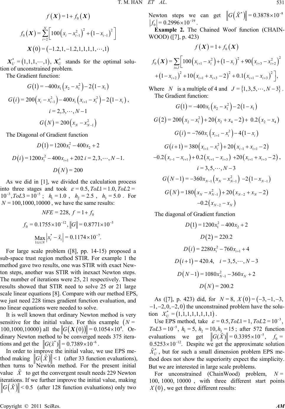

T. M. HAN ET AL.531

f

0
f=1
X
X


01
=100 1
N
i
fxx

 



X


2
i


2
1
i
x

2
=2
i
 
0=1.2,1,1.2,1,1,1, ,,1 X 1

*=1,1,1,,1 ,
UX* U
X
stands for the optimal solu-
.
The Gradient function:
x
tion of unconstraine d pr oblem



2
12 11
1= 40021Gxxx

 

22
1
= 20040021
ii i
Gixxx xxx

  ,
1 i ii
=2 ,3, i , 1 N



21
=200 NN GNx x 
The Diagonal of Gradient function

2
12
1 =12004002Dxx



21
=1200400202=2,,,1.
ii
Dix xiN

  3
As we did in [1], we divided the calculation process
into three stages and took

=200DN
= 0.5,1=1.0,2 =ToL ToL

, 2=2.5h, 3=5.0h. For
ve the me results:
35
10,3=10ToL

=100,1000, 100N; 1=1.0h 00 , we hasa
0
= 228,=1NFEf f
12
0= 0.175510,f

5 = 0.877110G


*7
= 0.117410.
ii
x 

1
Max
iNx 
For large scale problem ([8], pp. 115) proposed a
sub-space trust region method STIR. For examle 1 the
method gave two results, one was STIR with exNew-
ton steps, another was STIR with inexact Newton steps.
The number of iterations were 25, 21 respectively. These
re
4- p
act
sults showed that STIR need to solve 25 or 21 large
scale linear equations [8]. Compare with our method EPS,
we just need 228 times gradient function evaluation, and
no linear equations were needed to solve.
It is well known that ordinary Newton method is very
sensitive for the initial value. For this example

=N

100,1000,10000 all the
 
4
0= 0.105410.GX Or-
dinary Newton method to be converged needs 375 itera-
tions and get the *6 ()= 0.738910Gx   .
In order to improve the initial value, we use EPS me-
thod making

<1GX
 (after 33 function evalua,
wton mnitial
value
tions)
then turns to Neethod. For the present i
X
 to get the convergent result needs 229 Newton
iterations. If we further improve the initial value, making

<0.5GX
 (after 128 function evaluations) only two
ewton steps wegetN can

*8
= 0.387810

GX 

19
0= 0

.2996 10f
Exam The Cunction (CHAIN-
OOD, p. 42
.
ple 2.
) ([7]hained 3) Woof f W


0
=1ff
X
X




2
2
22
01 32
= 100190
ii iii
iJ
fxxxxx






X

222
213 13
110 20.1,
iiiii
xxx xx
 


Where N is a multiple of 4 and 5, ,3JN

= 1,3,

.
The Gradient function:





2
12 11
1=4002 1Gxxxx




2

21 24
2=20020 2Gxxxx




24
0.2
x
x





2
1
=760 41
ii ii
Gix xxx

 





2
11
1=380 202
ii ii
Gix xx x
 1

 




11 13
0.2
ii ii
xx xx
 
 13 20 ii xx

0.2

2 ,
=3,5, ,iN3




2
1 NNN
GNxx x

 
1

1
21 N x  1= 360





212
=18020 2
NNN N
GNx xxx





2
0.2
N
N
x
x


The diagonal of Gradient function


2
12
1 =12004002Dxx


2= 220.2D


21
= 22807604
ii
Dix x




1=420.4,= 3,5,,3Dii N




21
1 =10803602
NN
DNx x





= 200.2DN
As ([7], p. 423) did, for = 8, N
 
0=3, 1, 3,X


oblemave the solu-

1, 2,0, 2,0
tion the unconstrained pr h


,1,1,1,1,1.
thod, take 
*=1,1,1
U
X
Use EPS me3 1=1,2=10 ,ToL=0.5,ToL

5
3=10 ,ToL h
evaluations 1=5, we get
23
0, =15hh; after 572 function =1 5
()= 0.339510,GX  
0=f
12
0.5253 10.


*
U
Despite we get the approximate solution
X
, but for s
thod does nouch t sha small dimension ow the superiority expect t
problem EPS m
he simpe- licity.
But we are interested in large scale problems.
For unconstrained (ChainWood) problem,
, with three different start p=N
oints
100, 1000, 10000


0X, we get three different results:

T. M. HAN ET AL. 532
(the original)
1)
 
0=3, 1, 3, 1,X
Take 35 ,3=10 ,ToL

1=h5.

2,0,, 2,0
=0.5,1=1.0,2=10ToL ToL 
1 0h, after 811 function eva-
10000 , we get same appro-
f the minimal value of fu
5.0, 2=10.0h, 3=
ns, for = 100,1000, N
nction 0 =1 =ff
luatio
ximation o

113.808=14.808.

0=3, 1, 3, 1,0,0,,0,0 X
The parameters are the same as (1), for =100N,
after 857 function evaluations, we have ff
2)
 
0
=1=

10
1 0.18824 10. For =1000,1000 0 N after 856 f
we get the same result 0
=1 =ff
un-
ction evaluations,

10
9438 10 .
 
0=0, 1,0, 1,0,0,,0,0 ,
1 0.1
X
3)

0X is the
me this sa arameters are as [8].
The p
=.0,= 0.5.  For =100N,
after 628 fune have 0 =1 =ff
3
1=5.0,2 =10,3=ToL ToLToL

3
, =15h
aluations, w
512
10 ,2.0,=10.0hh

ction ev

13.5743 =4.5743, it is exactly consistent with STIR.
whHowever, SBMIM
coged to 46.713. For
ich STIR wanted to compare with,
=1000N, 10, [8] did not
nver 000
give terge. Ou
ons con
n and Y. H. Han, “Solving
tions by a New ODE Numerical Integration
3027
] P. Deuflhard, “Newton Methods for Nonlinear Problems
ce and Adaptive Algorithms,” Springer-
, 2004.
1996.
a
he results because SBMIM did not convr
method EPS, after 652, 659 function evaluati-
verged to the same result 4.5743.
7. References
[1] T. M. Ha Large Scale Nonlin-
ear Equa
Bou
Method,” Applied Mathematics, Vol. 1, No. 3, 2010, pp.
222-229. doi: 10.4236/am.2010.1
[2 Affine Invarian
Verlag, Berlin
[3] D. J. Higham, “Trust Region Algorithms and Timestep
Selection,” SIAM Journal on Numerical Analysis, Vol. 37,
No. 1, 1999, pp. 194-210.
doi:10.1137/S0036142998335972
[4] D. M. Young, “Convergence Properties of the Symmetric
and Unsymmetric Successive Overrelaxation Methods
and Related Methods,” Mathematics of Computation, Vol.
24, No. 112, 1970, pp. 793-807.
doi:10.1090/S0025-5718-1970-0281331-4
[5] Y. Saad, “Iterative Methods for Sparse Linear Systems,”
PWS Publishing Company, Boston,
[6] A. Miele and J. W. Cantrell, “Study on a Memory Gradi-
ent Method for the Minimization of Functions,” Journal
of Optimization Theory and Applications, Vol. 3, No. 6,
1969, pp. 459-470. doi:10.1007/BF00929359
[7] A. R. Conn, N. I. M. Gould and P. L. Toint, “Testing
Class of Methods for Solving Minimization Problems
with Simple Bounds on the Variables,” Mathematics of
Computation, Vol. 50, No. 182, 1988, pp. 399-430.
doi:10.1090/S0025-5718-1988-0929544-3
[8] M. A. Branch, T. F. Coleman and Y. Y. Li, “A Subspace,
Interior, and Conjugate Gradient Method for Large-Scale
nd-Constrained Minimization Problems,” SIAM Jour-
nal on Scientific Computing, Vol. 21, No. 1, 1999, pp.
1-23. doi:10.1137/S1064827595289108