Applied Mathematics, 2011, 2, 515-520
doi:10.4236/am.2011.25067 Published Online May 2011 (http://www.SciRP.org/journal/am)
Tail Behavior of Threshold Models with Innovations
in the Domain of Attraction of the Double
Exponential Distribution
Aliou Diop, Saliou Diouf
Laboratoire d'Etudes et de Recherche en Statistique et Développement,
Unité de Formation et de Recherche de Sciences Appliquées et Technologie,
Université Gaston Berger, Saint-Louis, Sénégal
Received February 15, 2011; revised March 6, 2011; accepted March 9, 2011
Abstract
We consider a two-regime threshold autoregressive model where the driving noises are sequences of inde-
pendent and identically distributed random variables with common distribution function which
belongs to the domain of attraction of double exponential distribution. If in addition,
,1,2
i
Fi


..
ir
F
Si  e



lime ,
iy
x
i
Fx y
Fx


 for each and
,x


lim :
ii
xi
i
FFx d
Fx
 


 where
F
*G denotes the con-
volution of the distribution function and 1,
F
F

 we determine the tail behavior of the process and give
the exact values of the coefficient.
Keywords: Tail Behavior, Domain of Attraction, Convolution Tails, Stochastic Recurrence Equation,
Threshold Autoregressive Model
1. Introduction
Switching regimes is stylized facts encountered in finan-
cial data analysis, concerning either financial returns, in-
terest rates or volatilities. The threshold autoregressive
(TAR) model was introduced by Tong [1] and has since
become quite popular in non-linear time series modeling.
The TAR model can be seen as a stochastic difference
equation. The tail behavior of a stationary solution of
such equation has been widely studied in a variety of
context.
A result of Kesten [2] shows that the stationary solu-
tion to the stochastic recurrence equation has regularly
varying distribution, under quite general conditions on
the multiplicative coefficient and the noise term. Davis
and Resnick [3] treat the bilinear process with regularly
varying innovations. Resnick and Willekens [4] consider
a stochastic recurrence equation with regularly varying
noise.
In these papers, either the multiplier in the stochastic
difference equation is a positive random coefficient or
the noise term is an independent and identically distri-
buted 

 valued random variable. Furthermore, in
general, the coefficient and the noise are assumed to be
independent. The latter condition is often not satisfied in
applications. Diop and Guégan [5] studied the threshold
autoregressive stochastic volatility model where the dri-
ving noises are sequences of independent and identically
distributed regularly varying random variables.
In our framework, the TAR model is a stochastic dif-
ference equation where the multiplicative coefficient and
the noise term are dependent. The random coefficient
model does not necessarily satisfy the positivity condi-
tion on the multiplier and the noise term. In addition, the
innovations are assumed to belong to the maximum do-
main of attraction of the double exponential distribution.
To our knowledge the literature is not abundant for this
framework.
A distribution function F is in the domain of attraction
of the extreme value distribution



exp e,
x
x  
x

 if there exists such that

1n0,
nn
ab

 
lim, .
n
nn
nFaxb xx 

  (1)

A. DIOP ET AL. 516
A distribution F is in the class

r
S

for 0

 if
for all x and

1Fx


lime ,
y
x
Fx y
Fx


 for each (2) ,y
and




12
1
*
lim lim:
xx
FFxX Xxd
FxX x
 





(3)
where 1
F
F and *
F
G denote the convolution of
the distribution function F and G. See Cline [6] and Em-
brechts [7] for further details on convolution tails. The
constant d is known to equal . In the sequel, we
set
1
2e
X 


eX
F
m

  when F is the distribution function
of the random variable X.
The aim of this paper is to study the tail behavior of a
two-regime threshold autoregressive model when the
driving noise of each regime has distribution function
 
,1,2
ir
FDS i   .
Let us give the motivation to justify why these results
are needed to be extended to the proposed class of resid-
ual processes. First, the distribution in


r
S

are
among others used to model claim size in risk theory
Klüppelberg [8], Beard et al.[9], Hogg and Klugman [10],
Goldie and Resnick [11]. Second,



r
SD

 is a
large class of distributions which constitute the domain
of attraction of mean residual lifetimes to the exponential
limit law whose behavior is preserved under convolu-
tions. In this paper, precisely we determine the exact
value of the coefficient in the tail behavior of the sta-
tionary solution when the model is stationary in some
regimes and mildly explosive in others.
The rest of this paper is organized as follows: Section 2
describes the model and conditions for strict stationarity are
provided. Some preliminary results with respect to the in-
novation processes are given. Section 3 presents the main
results.
2. The Model
The threshold autoregressive (TAR) model is defined by
the following relation


1
11 1
2
21 1
Φ,if
Φ,if
tt t
t
tt t
ZY
ZY













(4)
where

, are non random constants and with thre-
shold variable .
Φi
1t
Y
2.1. Assumptions
We will use the following assumptions.
H1-


 1
i
Z is sequence of independent and identically
distributed random variables (i = 1, 2) and satisfied the
following conditions:

1
log ,
i
Z




 (5)
where


logmax0, log.
x
x

H2- For each i = 1, 2, the two sequences of random
variables



i
tt
Z and


tt
Y are independent and



1
tt
Z and



t
2
t
Z are independent.
H3- The sequence of independent and identically dis-
tributed random variables
t
whose common dis-
tribution Fi is both in the domain of attraction of


i
t
Z




exp e,
x
x
x

  and in and
satisfies the tail balancing condition.

,
r
S  0









11
11
lim, lim1,
ii
ii
xx
ZxZ x
pp
Zx Zx
 






(6)
We define


,
t
Y



1
1t tY
1,I



21 1.
tt
I
I


Then Equation (4) can be rewritten as:

1
Φ,
tt tt
Z




 (7)
where

112 2
ΦΦ Φ
t ttt
I
I

 and
 
12
12
.
ttttt
Z
ZIZ I
We easily check that the tail balancing condition (6)
holds for random variables

k
Z
whose distribution
function


12
1
F
qFq F .
2.2. Preliminary Result
The Equation (7) is a stochastic difference equation
where the pair



Φ,t
tt
Z
are sequences of iid 2


values random variables under 1
H
and 2
H
. The next
proposition gives the strict stationarity of the process


tt

defined in (7). The result follows from Theorem 1
of Brandt [12].
Proposition 1 (strict stationarity) Assume 1
H
and
2
H
and suppose that 1
12
ΦΦ 1
qq. Then, for all
t

, the series


tt

defined in (7) admits the fol-
lowing expansion

1
00
,
j
t tk
jk
Z 
 
 





 t
j
(8)
which converges almost surely. Then the process


tt

is the unique strictly stationary solution of (7).
Proposition 2 Let

12
1.
F
qFq F
1) If


,1,2
i
FD i , then

.FD
2) If


,
ir
FS

 1, 2,0i


, then


.
r
FS


Proof

A. DIOP ET AL.517
Without loss of generality, we can assume that



2
1
,
F
x
F
x
tends to some constant as 0c
x
 which we
denote by 22
~
F
cF with Then the proof of 1)
follows from Proposition 3.3.28 of Embrechts and et al.
[13]. Indeed
0c

 


2
11
1,
F
xF
qq
x
F
xF
 x
which tends to some positive constant as 0 k
x

Hence F belongs to Now we prove 2).

D
First, using 21 ~
F
cF with , it is easy to show
by simple calculations that
0c


e,
y
Fx y
Fx

 as .
x

It suffices now to show that


*
lim .
x
FFx d
Fx



Now, we use the decomposition

 


 

 

 

12
11 12
2
12 12
21 22
2
12 12
1
(1 )(1 )
ZZ x
qZ ZxqqZ Zx
qqZZxqZZ x


 



Then



 

 


 

 


 

 



 

12
1
11 12
2
12 12
111 2
11 121211 1211
21 22
2
12 12
12 11
11 121111 1222
1
1(1)
ZZ x
Zx
qZZxq qZZx
IZ IZxIZ IZx
qqZ ZxqZZx
I
ZIZxIZIZ x


 

 
 

 







We can write








2
11 12
2
22
**2(1)*
(1 )*
F
FxqFFxqqFFx
Fx FxFx
qF Fx
Fx




（9）
where
 
12
1
F
xqFx qFx .
Since F1 and F2 belongs to the class

r
S

we have


11
1
1
*
lim
x
FFx d
Fx
 
and


22
2
2
*
lim .
x
FFx d
Fx
 
Then


 
2
11
21
*.
1
FFx qd
q
F
xqcq

Similarly, we have
 



22
22 2
1* 1
1
qFFx qcd
F
xqc

q
Using Theorem 1 of Cline [6], we show that
 

 

121 2
1* 1.
1
qqFFx qqdcd
Fxq cq



The proposition is entirely demonstrated.
3. Main Results
Our aim in this section is to establish the tail behavior of
the stationary distribution of


tt

defined in (4).
Theorem 1 Let


tt

be the stationary solution of
Equation (7) and the process t

t
Z
be an iid sequence
of random variables with common distribution




i
FD S
r

 satisfying (6). Suppose that the
assumptions of Proposition 1 hold. Then the tail behavior
of the stationary distribution of

tt

is





01 11()
***
0
1
1
12 1,
0
lim
ΦΦ ,
n
ii
t
t
x
n
iG
GG GG
i
n
in i
ni
i
x
Fx
mmm
mp























(10)
where



12,,
0
ΦΦ ,1
j
j
j
k
kjk kk
GFjk jkj
k
mm ppCq  q








01
***
i
GG G
can be computed using the following re-
cursion formula:
m








 
112
0
112
00
12
Φ1Φ
1
ii
FFF F
G
FF
GG G
mqmm qmm
mqmm qmm
 
 





0
i
(11)


i01
0** *
G
mi
GGG
m


 
and

A. DIOP ET AL. 518
 

  
12
1
11
21
1
12 1
12
if Φ1, Φ1,
δ1δ,ifΦ1, Φ1,
1ifΦ1, Φ1,
1δ1δ,ifΦ1, Φ1,
0, if
,
Φ,
,
Φ1, 1
k
k
kk
k
k
k
kk
q
pq pp
q
pqp p










 

 




2
(12)
with
1, if even
δ
0, if old
k
k
k


 (13)
Remark: We may give an financial example of model
(4) introduced by Breidt [14] for a financial return Yt
defined by the following relation
exp 2
t
t
Y

t





(14)
Where t

is an open-loop threshold autoregressive
process (Tong [15], p. 101)


1
11 1
2
21 1
Φ,if 0
Φ,if0
tt t
t
tt t
ZY
ZY










(15)
The model is called a threshold autoregressive sto-
chastic volatility model (TARSV). The log-volatility
process


tt

has a piecewise linear structure. It switches
between two first-order autoregressive process according
to the sign of the previous return. In this framework,

is positive constant and

t

t

is a sequence of inde-
pendent and identically distributed random variables
with zero mean and its variance is taken to be one. When
either 1 Φ1 and 2 Φ1 or 2 Φ1 and 1 Φ1

,
the process defined in (15) is stationary in some regimes
and mildly explosive in others. These models are sta-
tionary in some regimes and mildly explosive in others.
See Gongalo and Montesinos [16]. Gouriéroux and
Robert [17] studied the ACR(1) process where there is a
switching between white noise and a random walk.
Before proving Theorem1 we establish three lemmas.
The next lemma is due to Davis and Resnick [18]. Its
proof will then be omitted. The second lemma is an ex-
tension of Proposition 1.2 in Davis and Resnick [18]
where the hypothesis of independence is relaxed. See
also Cline [6]. They are needed for the proof of the tail
behavior of

t

.
Lemma 1
Suppose so the Balkema and de Haan[19]
representation holds

FD
 
0
1
expd ,
x
Z
F
xx t
ft








for some z0 and 0
x
z where



0,x   

0,z
as
is absolutely continous on ,xf 0

with
density f' and


'fulim 0
u

. Given 0

, there exists


00
xx

 such that for 0
x
x

 


1
1
1
1,
1
Fc xfx c
Fxx c





 



 


.
(17)
For any 01c


This following lemma is quite general since it does not
require the hypothesis of independent between the Yi’s.
Lemma 2
Let


,1
i
Yin


i
G
be random variables with distribu-
tion function and suppose

r
FS

. If



lim 0,
()
i
i
x
Yx
Fx







(18)
for 1,,in

 then for all , 2n



 
12 11
1
***
1
lim
ii n
n
i
i
x
n
iGGGGG
i
Yx
Fx
mmm












(19)
Proof
When 2n

, then this lemma is the formulation of
Theorem 1 of Cline [6]. When , set 1
and G its distribution function. Applying (19), when
2nn
i
i
SnY


2n

, we have






 
11
111
1
11
11
1
1
1
lim lim
.
iin
i
iin
n
i
inn
xx
n
nGiGG Gn
G
i
n
iGG
G
i
Yx SY
Fx Fx
mmmmm
mm m

 
 



 


















(20)
with


01
0** *
ii
GG G
G
mm


 
Lemma 3






1
10
Φ
lim 0.
j
tj
tk
jn k
xt
Zx
Zx



 





 (21)
Proof
For 0

 and for all b such that

1
1
1
1
1
Φ
b




,


(16)

A. DIOP ET AL.519
We have



1
10
12 ,
10
Φ
ΦΦ 1,
j
tj tk
jnk
j
kjk nj
tj jk
jn k
Zx
Z
bbxp


 



 












where

,1.
j
k
kk
jk j
pCq q


Using the tail balancing condition (6), we have







,
0
1
,
0
δδ
δ
δ
,
jtj ktj k
j
k
kt
tj k
j
k
jk
k
Zx Zx
p
Zx
Zx
Fx pp
Fx













where

1
12
δ1.
njk jk
kbb 

 Since
b
1, it is
readly seen that
b
1, for all. j > n and Hence
applying Lemma 1 with
.k
1
δk c

, given ε > 0, there ex-
ists 0
x
such that for 0
x
x, we have

 


1
1
1
,,
.
1
00
δδ
1
1δ
jj
kk
j
k
kk k
Fx fx
p
Fx x















 jk
p
Now following the proof of Proposition1.1 of Davis
and Resnick [18], we give an upper bound of
 
 
11
1
12 ,
10
1ΦΦ
j
njk jk
j
k
jn k
fx
K
bb p
x



 
 

 


 
Observe that

 


1
1
12 ,
0
11
(1)
1ΦΦ
1Φ
j
njk jk
j
k
k
j
n
bb p
bb b


















This implies





1
10
12
10
1
1
1
1
Φ
ΦΦ 1
Φ.
j
tj
tk
jnk
j
kjk nj
tj
jn k
j
jn
Zx
Z
bbx
fx
Kb
x








 





















Since

 
1
1
Φ1andlimlim0
xx
fx
bf
x

 x


The result follows.
Proof of Theorem 1
Set

1
00
Φ,
j
n
nt tk
jk
SZ

 




 j
j
j
j
p

1
10
Φ,
j
nt
tk
jnk
RZ










1
0
Φ.
j
nt tk
k
YZ

 






Denote by Gj the distribution function of Yj. First, it is
easy to check that the moment generating function Yj
exists and is given by


12 ,
0
ΦΦ
j
j
iji
GF
i
mm 


i
Next note that

11
ΦΦΦ
ntttntn
R




  1
Φ,Φ,,Φ
tt t

. Using
the independence between and


n

1tn



, we can compute the moment generating func-
tion of which we denote by
n
Rn
R
m,



1
1
1
12 1,
0
ΦΦ
ntn
n
in i
R
ni
i
mm



 p



where t m

is the moment generating function of t

.
By the stationarity of


t

, we get


1
12 1,
0
ΦΦ
nt
in i
1n
R
ni
i
mm







p
Using the rapidly variation of
F
and the tail
balancing condition (6), we can establish that





12
,
0
lim
ΦΦ
lim
i
x
kjk
jtj
j
k
xk
j
Yx
Fx
Zx
p
Fx




 







(22)
j

is given by (12).
By Lemma 2, we have



 
12 11
***
1
lim
ii n
n
x
n
iGGGGG
i
Sx
Fx
mmm









(23)
Moreover, by lemma 3

A. DIOP ET AL. 520


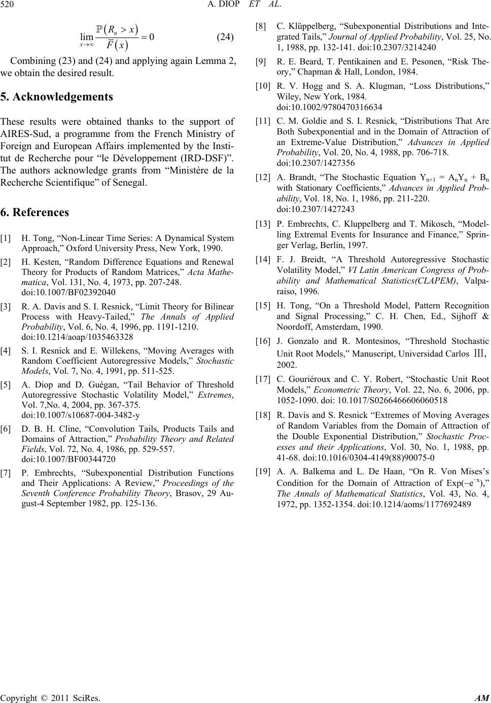
lim 0
n
x
Rx
Fx

 
(24)
[8] C. Klüppelberg, “Subexponential Distributions and Inte-
grated Tails,” Journal of Applied Probability, Vol. 25, No.
1, 1988, pp. 132-141. doi:10.2307/3214240
Combining (23) and (24) and applying again Lemma 2,
we obtain the desired result.
[9] R. E. Beard, T. Pentikainen and E. Pesonen, “Risk The-
ory,” Chapman & Hall, London, 1984.
[10] R. V. Hogg and S. A. Klugman, “Loss Distributions,”
Wiley, New York, 1984.
doi:10.1002/9780470316634
5. Acknowledgements
These results were obtained thanks to the support of
AIRES-Sud, a programme from the French Ministry of
Foreign and European Affairs implemented by the Insti-
tut de Recherche pour “le Développement (IRD-DSF)”.
The authors acknowledge grants from “Ministère de la
Recherche Scientifique” of Senegal.
[11] C. M. Goldie and S. I. Resnick, “Distributions That Are
Both Subexponential and in the Domain of Attraction of
an Extreme-Value Distribution,” Advances in Applied
Probability, Vol. 20, No. 4, 1988, pp. 706-718.
doi:10.2307/1427356
[12] A. Brandt, “The Stochastic Equation Yn+1 = AnYn + Bn
with Stationary Coefficients,” Advances in Applied Prob-
ability, Vol. 18, No. 1, 1986, pp. 211-220.
doi:10.2307/1427243
6. References
[13] P. Embrechts, C. Kluppelberg and T. Mikosch, “Model-
ling Extremal Events for Insurance and Finance,” Sprin-
ger Verlag, Berlin, 1997.
[1] H. Tong, “Non-Linear Time Series: A Dynamical System
Approach,” Oxford University Press, New York, 1990.
[14] F. J. Breidt, “A Threshold Autoregressive Stochastic
Volatility Model,” VI Latin American Congress of Prob-
ability and Mathematical Statistics(CLAPEM), Valpa-
raiso, 1996.
[2] H. Kesten, “Random Difference Equations and Renewal
Theory for Products of Random Matrices,” Acta Mathe-
matica, Vol. 131, No. 4, 1973, pp. 207-248.
doi:10.1007/BF02392040
[15] H. Tong, “On a Threshold Model, Pattern Recognition
and Signal Processing,” C. H. Chen, Ed., Sijhoff &
Noordoff, Amsterdam, 1990.
[3] R. A. Davis and S. I. Resnick, “Limit Theory for Bilinear
Process with Heavy-Tailed,” The Annals of Applied
Probability, Vol. 6, No. 4, 1996, pp. 1191-1210.
doi:10.1214/aoap/1035463328 [16] J. Gonzalo and R. Montesinos, “Threshold Stochastic
Unit Root Models,” Manuscript, Universidad Carlos Ⅲ,
2002.
[4] S. I. Resnick and E. Willekens, “Moving Averages with
Random Coefficient Autoregressive Models,” Stochastic
Models, Vol. 7, No. 4, 1991, pp. 511-525.
[17] C. Gouriéroux and C. Y. Robert, “Stochastic Unit Root
Models,” Econometric Theory, Vol. 22, No. 6, 2006, pp.
1052-1090. doi: 10.1017/S0266466606060518
[5] A. Diop and D. Guégan, “Tail Behavior of Threshold
Autoregressive Stochastic Volatility Model,” Extremes,
Vol. 7,No. 4, 2004, pp. 367-375.
doi:10.1007/s10687-004-3482-y [18] R. Davis and S. Resnick “Extremes of Moving Averages
of Random Variables from the Domain of Attraction of
the Double Exponential Distribution,” Stochastic Proc-
esses and their Applications, Vol. 30, No. 1, 1988, pp.
41-68. doi:10.1016/0304-4149(88)90075-0
[6] D. B. H. Cline, “Convolution Tails, Products Tails and
Domains of Attraction,” Probability Theory and Related
Fields, Vol. 72, No. 4, 1986, pp. 529-557.
doi:10.1007/BF00344720
[19] A. A. Balkema and L. De Haan, “On R. Von Mises’s
Condition for the Domain of Attraction of Exp(–e–x),”
The Annals of Mathematical Statistics, Vol. 43, No. 4,
1972, pp. 1352-1354. doi:10.1214/aoms/1177692489
[7] P. Embrechts, “Subexponential Distribution Functions
and Their Applications: A Review,” Proceedings of the
Seventh Conference Probability Theory, Brasov, 29 Au-
gust-4 September 1982, pp. 125-136.