 Journal of Computer and Communications, 2014, 2, 112-120 Published Online July 2014 in SciRes. http://www.scirp.org/journal/jcc http://dx.doi.org/10.4236/jcc.2014.29015 How to cite this paper: Wang, Z., Zhang, H.J. and Bi, G.A. (2014) Speech Signal Recovery Based on Source Separation and Noise Suppression. Journal of Computer and Communications, 2, 112-120. http://dx.doi.org/10.4236/jcc.2014.29015 Speech Signal Recovery Based on Source Separation and Noise Suppression Zhe Wang, Haijian Zhang, Guoan Bi School of Electrical and Electronic Engineering, Nanyang Technological University, Singapore Email: wang0755@e.ntu.edu.sg, zhaijian@ntu.edu.sg, egbi@ntu.edu.sg Received May 2014 Abstract In this paper, a speech signal recovery algorithm is presented for a personalized voice command automatic recognition system in vehicle and restaurant environments. This novel algorithm is able to separate a mixed speech source from multiple speakers, detect presence/absence of speakers by tracking the higher magnitude portion of speech power spectrum and adaptively suppress noises. An automatic speech recognition (ASR) process to deal with the multi-speaker task is designed and implemented. Evaluation tests have been carried out by using the speech da- tabase NOIZEUS and the experimental results show that the proposed algorithm achieves impres- sive performance improvements. Keywords Speech Recovery, Tim e-Frequency Source Separation, Adaptive Noise Suppression, Automatic Speech Recognition 1. Introduction In ubiquitous environment of multiple speakers, it has been a challenge to adapt the speech recognition model correctly for improving the speech recognition accuracy. The recovery of clean speech from a noisy resource is of vital importance for speech enhancement, speech recognition and many other speech related applications. In real life, there are numerous noise sources such as environment, channel distortion and speaker variability. Therefore, many algorithms have been reported for removing the noise from speech. Most of these algorithms need additional noise estimation and are only adapted to auditory effect rather than the ASR. This paper de- scribes a novel self-optimized voice activity detection (VAD) algorithm together with a simple but effective noise removing process after signal separation for improving speech recognition rate. The key feature of the pro- posed VAD algorithm is that prior estimation of clean speech variance is not needed. In addition, the threshold used for speech/non-speech decision is generated from the noisy speech itself, which is considered as a kind of self-optimizing process. For the noise removing process, the key feature is the simplicity because it is based on the widely known spectral subtraction (SS) [1] method without any additional model or training process. Per- formance comparison has been made among SS method [2], zero-cros si ng-energy method (ZCE) [3], entropy- based method [4], and the proposed VAD based algorithm.  Z. Wang et al. To perform the recognition task simultaneously, a modified recognition speaker process based on Bhattacha- ryya distance is proposed to process the separated speech for isolate word recognition. In this recognition scena- rio, the computational complexity is not increased in proportion to the number of template words from multiple speakers. Experimental results based on the noise and speech from the NOIZEUS database show the desirable performance. The rest of the paper is organized as follows. In Section 2, a speech separation process is described to obtain individual signals from the noisy voice of multiple speakers without knowing the number of speakers. In Section 3, the self-optimized VAD algorithm is presented with detailed derivation steps. Section 4 provides an adaptive soft decision algorithm for noise suppression. Section 5 presents the modified Mel Frequency Cepstrum Coeffi- cient (MFCC) based ASR system used in the multi-speaker adaption experiment. The experimental results and the performance comparison among various reported methods are presented in Section 6. Conclusions are given in Section 7. 2. Blind Source Separation (BSS) Based on SSTFT Assume Sn(t), n = 1, …, N, be the unknown speech sources, where N is the number of speakers. The arrange- ment of an M-sensor microphone array is linear. The output vector is modeled as (1) where A denotes the mixing matrix, x(t) = [x1(t), …, xM(t)]T is the vector of the received mixtures, s(t) = [s1(t), …, sN(t)]T contains the multiple speech sources, n(t) is the additive white noise vector and T is the trans- pose operator. The procedure of the spatial short-time Fourier transform (SSTFT) BSS algorithm based on the above signal model is presented as follows: • Calculating the STFT of the mixtures x(t) in (1), we obtain an M × 1 vector at each time-frequency (TF) point as ()() ()t, ft, ft, f= + x sn SAS S (2) where the subscript, S, denotes the STFT operator. • Next, we detect the auto-source TF points, i.e. the auto-term location of the speech sources in TF domain based on the criterion at each time-instant 0 ||S(t,f) ||/ max||S(t,v) || xvx >ε (3) where ||•|| denotes the norm operator and is an empirical threshold value for selection of the auto-source TF points. All the TF points which satisfy the criterion in (3) are included in the set Ω. • The premise of the SSTFT-based algorithm is to estimate the number of sources N as well as the mixing ma- trix A. We apply the method proposed in our previous work [5]. Specifically, we try to detect some domi- nant TF points, i.e., the points at which one of the sources has the dominant energy compared to those of other sources and noise power. The mean-shift clustering method [6] is applied to classify the dominant TF points without knowing the number of sources. The mixing matrix A is estimated by averaging the spatial vectors of all TF points in the same cluster, and N is estimated by counting the number of resultant clusters. • Based on the detected auto-source TF point set Ω and the estimated mixing matrix A, we can apply the sub- space-based method to estimate the STFT values of each source [7]. We assume that there are at most K < M sources present at each auto-source TF point ∈ Ω. Thus, the expression in (2) is simplified as () (),()t, ft, ft, f≈ ∈Ω xS S AS (4) • where denotes the steering vectors of the K sources at each point , and contains the STFT values of these K sources. at each auto-source TF point can be determined by the following mi- nimization ,, 1 ˆ ˆ ..., X arg{PS ()} mm K aa t, f=A (5) where 1 (AA )A HH m mmm − = −PIA denotes the orthogonal projection matrix into noise subspace, where contains the random K columns of the estimated mixing matrix A. The K STFT values at 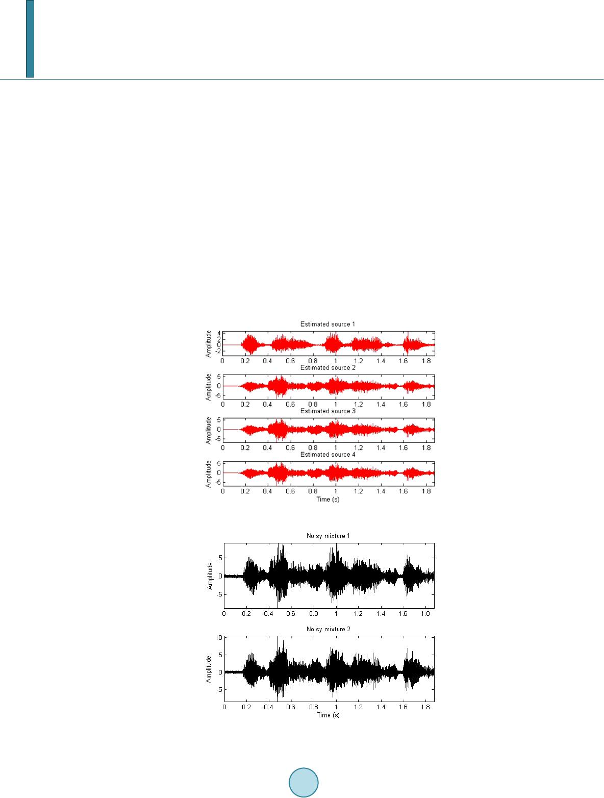 Z. Wang et al. each auto-source TF point can be obtained by † ()A (),()t, ft, ft, f≈ ∈Ω Sx SS (6) where † denotes the Moore-Penrose’s pseudo inversion operator. Now the energy at each auto-source TF point in Ω is separated into K STFT values assigned to corresponding sources. • Each source is recovered by the inverse STFT [8] using the estimated STFT values by (6). Figure 1 presents the results of using the above presented process for separating four speakers’ voices from the signals received by two microphones, as seen in Figure 2. 3. Noise Estimation Noise and speech are usually statistically independent and possess different statistical properties. Noise is more symmetrically distributed and present all the time, while speech is frequently non-stationary due to its active/ non-active periods. The active/non-active transition of speech makes the energy of speech more concentrated in the speech active period. 3.1. General Description The different behaviors of noise and speech make it possible to track speech or noise based on the minimum/ Figure 1. Separated voices from four speakers. Figure 2. Mixed speech signals received by two microphones.  Z. Wang et al. maximum of speech spectrum. The part having high energy is more likely to be speech while the part with low energy is more likely to be noise, which makes it possible to detect speech by analyzing the maximum of noisy speech. The speech amplitude is more probably larger than the noise amplitude. Compared with noise, the probability distribution function of clean speech magnitude is flatter in the “tail” part, which means clean speech magnitude is more likely far from its average. Even for SNR = 0 dB, the peak portion of the signal can be prov- en to be more likely from speech. 3.2. Algorithm Derivation Assuming that speech is distorted by uncorrelated additive noise, two hypotheses for VAD are : speech absent: Y = N + R : speech present: Y = S + N + R where Y, N, S, and R denote the frequency domain noisy speech, noise, clean speech and residual speech from the source separation process, respectively. The probability density function for H0 and H1 are given by ( ) ( ) 2 2 00 22 2 : ()2 N N NR Y exp HPYf YH σ πσ σ − == + (7) ( ) ( ) 2 222 11 222 2 : ()()2 NRS NRS Y exp HPYfYH σσσ πσσ σ −++ = =++ (8) where , and denote the noise, residual and clean speech variance. We have the conditions and , where is a heuristic parameter between 0.01 and 0.2. Its calculation will be further presented in Section 4. The first condition is simplified into ( ) 222 2 22 22222 11 exp 2 SNR NR NRNRS Y σσσ ε σσ σσσσσ ++ −< ++ ++ (9) Define , then ( ) ()( ) 2 22 1exp 2 21 NR Y kk k ε σσ + −+< ++ (10) or equivalently, ( ) ( ) ( ) 1 22 22 1 exp 1 21 k NR Y k k ε σσ + −< + ++ (11) From (11), we have ( ) 22 2 2 21 ln 21 SNR Ykk σσσε ++ >− ++ (12) Then define ( ) 22 2 2 21 ln 21 SNR Ykk ε σσσε ++ = − ++ (13) where can be served as a more direct threshold. Then the frequency bin level VAD flag can be achieved by 2 2 2 2 1, flag 0, YY YY ε ε > =≤ (14)  Z. Wang et al. The speech probability density function is calculated, which can be used to get . Then, the binary VAD flag can be achieved by using (13). The VAD algorithm mentioned previously is suitable on suppressing the noise and can effectively distinct the noise and voiced speech. To improve the auto speech recognition rate, we still need to trace changes in the noise-energy and update the noise energy in all frames including the speech frames. 4. Noise Suppression In the design of VAD algorithm, the soft decision algorithms appear to be superior to binary decision because speech signal is highly non-stationary. There is no clear boundary which marks the beginning or ending of a pronunciation. In this section, the discrimination information is used as a soft decision threshold. 4.1. Sub-Band Energy Calculation The energy calculation works on a frame by frame basis. Each frame is multiplied by a suitable window to re- duce the frequency aliasing from fast Fourier Transform (FFT). Note that the 50% overlapping means an initial delay of one half of the frame size is incurred. The frame size should be selected carefully. Suppose the sample rate is and frame size is N = 2m. The time resolution is N/Fs, and frequency resolution is Fs/N. Obviously a larger frame size allows better frequency resolution but has a poor time resolution. In general, for Fs = 8000 and 16,000 Hz, frame sizes of N = 256 and 512 are found appropriate, respectively. The signal is divided into 16 sub-bands. When the frame size is 256, the energy for the ith band is (15) where is the absolute value of the Fourier transform coefficient of the band. The sub-band out of the whole energy is calculated by (16) The frame energy and the sub-band energy are used to calculate the discrimination information based on the sub-band energy distribution probabilities for both the current frame and the noise frame. Assume the random variable Y has the chance to be a value of . The probability distribution of Y is related to the hypothesis H0 and H1. Set P0(αk) = P(αk|H0), P1(αk) = P(αk|H1), the discrimination information is defined as follows, 1011 0 1 (,;)()log[()/()] K k kk k IPPYPaPa Pa = = ∑ (17) The discrimination information can be calculated using sub-band energy distribution to measure the similarity of current frame and the noise frame. (18) (19) 4.2. Threshold Update The threshold value is updated by: • The first 5 frames are selected as the noise/non-speech frames. • The previous frame of a period of speech signal is considered as noise frame. • When the previous frame is considered as a noise frame, the current frame will be considered as noise frame if current frame satisfies |Y|2 ≤ |Yε|2. If the current frame satisfies |Y|2 > |Yε|2 and d > Tr, the current frame is considered as the start position frame and comparing with the next 6 frames is made. If the 6 frames also sa- tisfy |Y| 2 > |Yε|2 and d > Tr, the start position frame can be taken as the start position of a period of speech. Otherwise the current frame is still considered as a noise frame. • When the previous frame is a speech frame, if current frame satisfies |Y|2 > |Yε|2, it remains to be the speech  Z. Wang et al. frame. If the current frame satisfies |Y|2 ≤ |Yε|2 and d < Tr, it is classified as the end position frame, and then comparison with the next 6 frames is made. If the 6 frames also satisfy |Y|2 ≤ |Yε|2 and d < Tr, the end posi- tion frame can be taken as the end position of a period of speech (also the start point of a speech); otherwise, the current frame is still a speech frame. Tr is the edge value of the discrimination information which equals to the average discrimination value of the most recently 5 noisy frames. • During each step of the above determination, the noise threshold will be updated by (20) where represents the updated noise threshold for the nth frame, |Y|2 is the probability distribution function value of current speech and λ is the noise update factor, which is calculated by discrimination in- formation. • If all the data have been dealt with, the adaptive adjustment will end. 4.3. Modified VAD and Noise Suppression The speech signal Y(w) is generally corrupted by the additive noise, N(w), which is assumed to be independent of speech. In theory, the noise can be optimally removed by estimating its power and filtering the noisy signal with the following filter: (21) The proposed VAD will detect the noise frame, and subtract noise spectra from speech signal, trying to keep more information used during the feature extraction process of ASR and eliminating noise that provides wrong information during feature extraction and template matching. As the speech signal is always non-stationary, making a binary decision of being voice or noise is quite risky. Therefore, we have designed a module that rates the likelihood of voice by computing a voice activity score (VAS). In this way, we can achieve smooth process- ing transition when the derived VAS indicates a mixture of voice and noise. The VAS for a frame is determined by two aspects. The first one concerns with the intelligibility of the voice, which is approximately quantified by counting the number of Bark bands in the speech band whose power, ex- ceeds that of the corresponding Bark band of the estimated noise. The speech band ranges from the 4th to the 14th Bark band. The second aspect is the relative power of the current frame to that of the estimated noise power. In general, the higher the relative power of a frame, the more likely it contains voice. The final VAS is simply the sum of the scores from the two aspects. The parameter is set as the reciprocal of VAS and is updated for each frame. The continuous VAS offers much more flexibility than a fixed parameter. Even when it is necessary to make a binary decision as to whether or not the frame is a noise-only frame, we can still make the processing changing and converging at certain value. Then for each frame, the process described in Section 3.2 is conducted. With the processed results, and mentioned in Section 3.2 are updated correspondingly. 5. Speaker and Speech Recognition This section elaborates the full system from the front end feature extraction, training process which consists of sub-word unit and word template generation, and the final recognition process. After VAD and noise suppres- sion, the processed speech signal will be evaluated in this ASR system. 5.1. Front end Feature Extraction The feature vector used for this recognition task is 24MFCC. The frame window size is 20 ms and the speech is sampled at 16 kHz with 16 bit resolution. 5.2. Sub-Word Unit Generation The first part of the training process requires the users to record approximately two minutes of their speech. It is recommended to read phonetically rich sentences in order to obtain a more comprehensive sub-word unit. In this experiment, the user is asked to read a series of Harvard sentences. Then, the resulting MFCC is clustered by using c-means algorithm into 64 distinct units, roughly corresponding to a collection of sub-word. Each of these 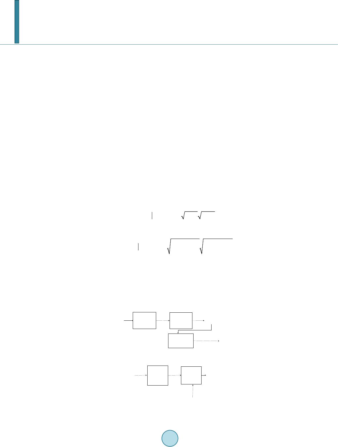 Z. Wang et al. clusters is then modeled using Gaussian mixture model of 4 mixtures. In this experiment, re-clustering is not done during word template generation. To simplify the model, further calculation is performed to generate the 64 by 64 Bhattacharyya distance matrix. This process is illustrated in Figure 3. 5.3. Word Template Generation In this step, the words to be recognized are registered. As shown in Figure 4, the user is asked to pronounce the words, and the template generation converts those words into a sequence of sub-word unit index (obtained from the previous step) based on its maximum likelihood. To avoid over segmentation of the word, transitional heu- ristic is employed by allowing the change of sub-word index only when there is a significant margin of likeli- hood difference with the neighboring state. This process has to be repeated for each word that the user wants to introduce to the system. 5.4. Matching Process—Recognition Assuming there are M word templates in the system, the recognition process calculates the probability of the us- er input feature vector X input being generated by the template. The chosen word is the one which gives the highest likelihood. (22) Note that the template can be viewed as a sequence of Gaussian Mixture Models (GMM), which makes the pm(XInput) calculation increasingly expensive with an increasing number of word templates and very hard to ob- serve the effect of proposed VAD algorithm [9]. We propose to convert the input feature to a sub-word unit in- dex sequence using the Bhattacharyya distance. The Bhattacharyya between two probability distribution and is defined by ( ) ( ) 121 2 Bln() ()hattpppxpx dx= − ∫ (23) Each sub-word unit in the testing experiment is modeled by using 4 mixtures GMM, so the distance between them is given by: ( ) 33 1 21,2, 00 Bln() () mix mix mix mix hattpppxpxdx = = = − ∑∑ ∫ The distance is calculated for all 64 sub-word units using Levenshtein distance method. The average run time of the recognition task by original pattern matching algorithms increases proportionally with the number of tem- plates. For the Bhattacharyya edit distance method, however, the running time is quite stable when the number of templates increases, which is particularly suitable for a real-time recognition system. Figure 5 shows his matching process. The speaker recognition process is similar to the matching process with two main differences. Firstly, only the selected speaker profile is loaded during word recognition process because at this point, the identity of the Figure 3. Sub-word unit generation. Figure 4. Word template generation. Front End Feature extraction Clustering and GMM modelling MFCC Speaker's Speech 64 Subword Unit (each modelled with GMM) Calculate Bhattacharyy a Distance 64 x 64 Distance matrix Front End Feature extraction Find Optimum Sequence MFCC Word1 Speech 64 Subword Unit Word1 Template (Subword Unit/GMM sequence) 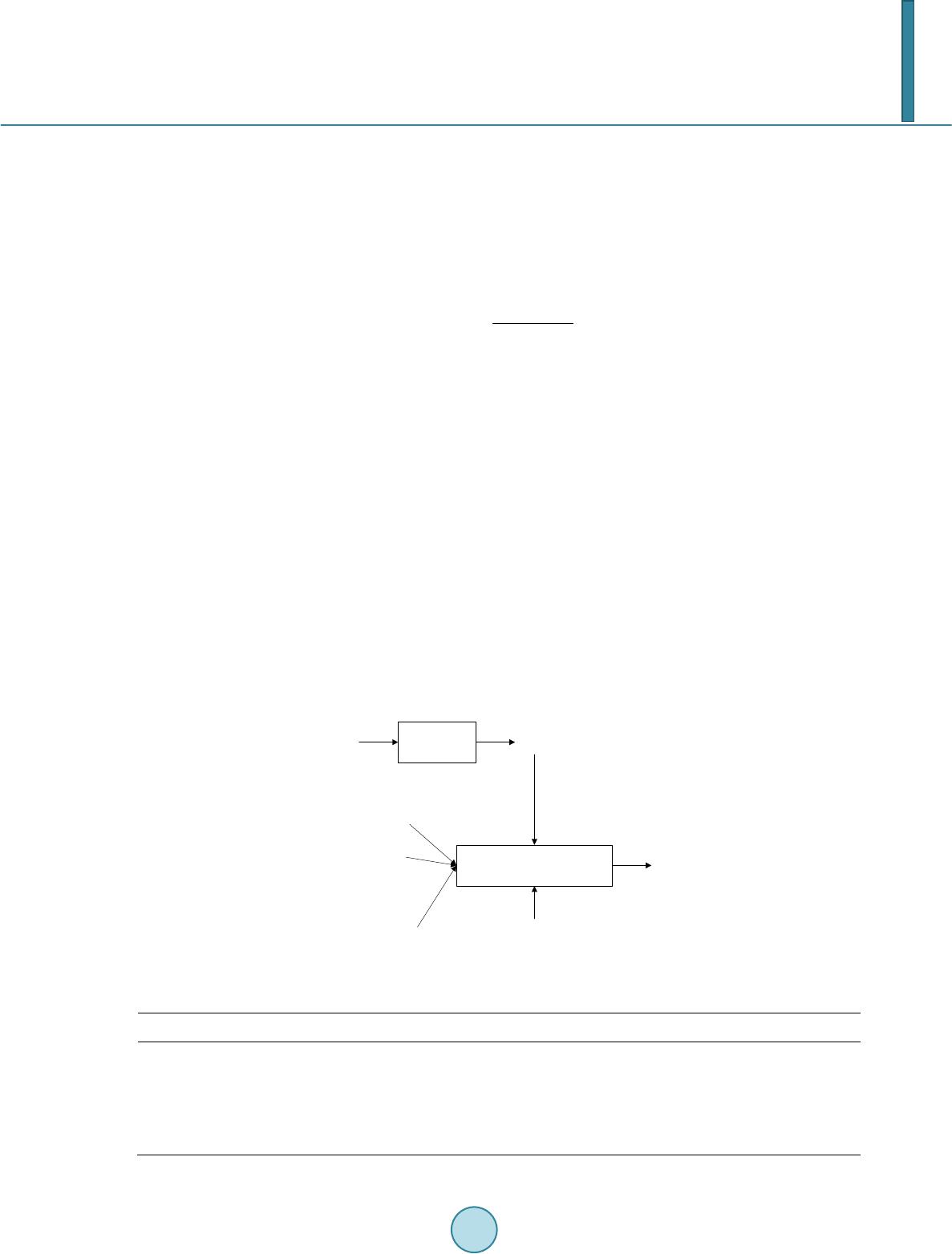 Z. Wang et al. speaker is already known. In speaker recognition, the speaker profile is polled and the input is compared against the respective activation keyword registration for each speaker. Secondly, instead of using edit distance, the speaker recognition process uses the posterior probability of the input given the sequence of GMM distribution in the template. This method gives us more flexibility in setting the threshold of acceptance. 6. Algorithm Evaluation In this section we present the results and an objective evaluation of the proposed ASR system. We define ( ) ( ) 12 0 12 0 10log n k n k Sk SNR Nk − = − = = ∑ ∑ (25) where S(k) is the speech signal energy and N(k) is the noise energy. In this ASR experiment, the noise of vehicle motor and restaurant are from NOIZEUS noise database [10]. Speech Recognition Tests Speech recognition test is carried out using ASR system in Section 5. The proposed blind source separation is imp lemented before VAD algorithm. In general, better separation results are achieved for the system with fewer speech sources than microphones [5]. In our case, we use 2 microphones to receive the mixed voices from 4 speakers. In the separated signals, one speaker’s voice is selected by using automatic speaker recognition and then conducted the isolate word recognition test. The performances from SS method, ZCE method, and Entropy- Based method are compared with that from the proposed VAD noise suppression method in motor and restau- rant noisy environments. Experimental results on accuracy are given in Tab l e 1 for the situations of SNR = 0, 5 and 10 dB. The recognition ratios under restaurant noise environment are given in parentheses. Compared with entropy-based method that achieves the most accuracy among VAD algorithms, the relative improvement in the case of SNR = 0 dB reaches 2.5% (1.2%), while in the case of SNR = 5 dB, the rate im- provement is 1.4% (0.33%). The entire ASR system works in a frame-by-frame manner and meets the real-time operation for most embedded electronic applications. In addition to the noise used in the experiment, the similar results are achieved by using street noise from NOIZEUS. Figure 5. Pro p osed method for word recogn ition . Table 1. Accuracy in vehicle motor and restaurant noise. SNR 0 dB 5 dB 10 dB SS 60.43(58.33) 79.86(75.94) 92.23(88.01) ZCE 76.77(70.52) 85.42(79.41) 93.91(87.68) Entropy-Based 84.09(83.56) 87.18(85.09) 93.95(91.82) Proposed VAD 86.59(84.72) 88.53(85.42) 93.98(92.08) Input Speech Word Template Generation Input Word Template Find Minimum Edit_distance(input,Word_x) Word1 Template Word2 Template Word100 Template ............ Output Word Distance Matrix  Z. Wang et al. 7. Conclusion In this paper, a complete speech recovery algorithm is proposed and implemented for ubiquitous speech envi- ronment. It can effectively recover the voice of individual speaker from mixed voice of multiple speakers in noisy environment. The key feature of the proposed algorithm is that the prior information on the number of sources and estimation of clean speech variance is not needed. The threshold used to suppress noise is generated from the speech itself, which leads to the desirable ability of adapting to changing environments. Moreover, the proposed source separation and noise suppression method does not need any additional training process, which effectively reduces the computational burden. Finally, the proposed system can be easily realized in ubiquitous environment. Acknowledgements The authors would like to thank STMicroelectronics Asia Pacific Pte Ltd for providing speech dataset and expe- riment environment. References [1] Boll, S. (197 ) Suppression of Acoustic Noise In Speech Using Spectral Subtraction. IEEE Transactions on Acoustics Speech and Signal Processing, 27, 113-120. http://dx.doi.org/10.1109/TASSP.1979.1163209 [2] Junqua, J.C., Mak, B. and Reaves, B. (19 94) A Robust Algorithm forward Boundary Detection in the Presence of Noise. IEEE Transactions on Speech and Audio Processing, 2, 406-421. http://dx.doi.org/10.1109/89.294354 [3] Beritelli, F., Casale, S., Ruggeri, G., et al. (2002 ) Performances Evaluation and Comparison of G.729/AMR/Fuzzy Voice Activity Detectors. IEEE Signal Processing Letters, 9, 85-88. http://dx.doi.org/10.1109/97.995824 [4] Abdallah, I., Montresor, S. and Baudry, M. (1997) Robust Speech /Non-Speech Detection in Adverse Conditions Using an Entropy Based Estimator. International Conference on Digital Signal Processing, Santorini, 757-760. [5] Zhang, H., Bi, G. , Razul, S.G. and See, C.-M. (2013 ) Estimation of Underdetermined Mixing Matrix with Unknown Number of Overlapped Sources in Short-Time Fourier Transform Domain. IEEE ICASSP, 6486-649 0 . [6] Co maniciu, D. and Meer, P. (2002) Mean Shift: A Robust Approach toward Feature Space Analysis. IEEE Transac- tions on Pattern Analysis and Machine Intelligence, 24, 603-619. http://dx.doi.org/10.1109/34.1000236 [7] Ai s sa-El-Bey, A., Linh -Trung, N., Abed-Meraim, K. and Grenier, Y. (2007) Underdetermined Blind Separation of Nondisjoint Sources in the Time-Frequency Domain. IEEE Transactions on Signal Processing, 55, 897-907 . http://dx.doi.org/10.1109/TSP.2006.888877 [8] Griffin, D. and Lim, J.S. (1984 ) Signal Estimation from Modified Short-Time Fourier Transfo rm. IEEE Transactions on Acoustics Speech and Signal Processing, 32, 236 -243. http://dx.doi.org/10.1109/TASSP.1984.1164317 [9] Chang, H.Y., Lee, A.K. and Li, H.Z. (2009 ) An GMM Supervector Kernel with Bhattacharyya Distance for SVM Based Speaker Recognition. IEEE ICASSP, 4221-4224. [10] Hu, Y. and Loizou, P. (2006) Subjective Comparison of Speech Enhancement Algorithms. IEEE ICASSP, 1, 153-156 .
|