American Journal of Computational Mathematics, 2014, 4, 223-232
Published Online June 2014 in SciRes. http://www.scirp.org/journal/ajcm
http://dx.doi.org/10.4236/ajcm.2014.43019
How to cite this paper: Ahmad, I. and Bilal, M. (2014) Numerical Solution of Blasius Equation through Neural Networks
Algorithm. American Journal of Computational Mathematics, 4, 223-232. http://dx.doi.org/10.4236/ajcm.2014.43019
Numerical Solution of Blasius Equation
through Neural Networks Algorithm
Iftikhar Ahmad, Muhammad Bilal
Department of Mathematics, University of Gujrat, Gujrat, Pakistan
Received 5 May 2014; revised 5 June 2014; accepted 11 June 2014
Copyright © 2014 by authors and Scientific Research Publishing Inc.
This work is licensed under the Creative Commons Attribution International License (CC BY).
http://creativecommons.org/licenses/by/4.0/
Abstract
In this paper mathematical techniques have been used for the solution of Blasius differential equ-
ation. The method uses optimized artificial neural networks approximation with Sequential Qua-
dratic Programming algorithm and hybrid AST-INP techniques. Numerical treatment of this prob-
lem reported in the literature is based on Shooting and Finite Differences Method, while our ma-
thematical approach is very simple. Numerical testing showed that solutions obtained by using the
proposed methods are better in accuracy than those reported in literature. Statistical analysis
provided the convergence of the proposed model.
Keywords
Blasius Equation, Neural Networks, Log-Sigmoid Function, Boundary Value Problems
1. Introduction
Blasius differential equation is the mother of all boundary layer equations in fluid mechanics. It is almost a
hundred-year-old differential equation and still an active topic among the all time researchers. Blasius derived
the famous Blasius equation by using transform technique. Equation was discussed in many articles by analy-
tical and numerical ways. Many scientists investigated interesting results of Blasius equation either from
mathematical point of view or from engineering prospective. Howart numerically solved this differential equa-
tion and com- pared the results w ith [1]. Further, analytical solu tions which are uniformly valid over the whole
domain do not exist till 1999. Liao in his best paper gave the result by Homotopy Analysis Method (HPM) [2]
[3]. G.I. Shishki n [4] showed asymptotic behavior of differential and difference solutions to get different scheme
with a finite number of nodes for enough long interval. The standard non-homogenous Blasius equation is
( )( )
12 0uxux
′′′ ′′ +=
; with the initial and boundary condition
( )
00u=
,
( )
0u α
′=
and
( )
1u∞=
, where
( )
ux
is dimension less stream function and is the similarity ordinate.

I. Ahmad, M. Bilal
224
The Blasius equation describes the velocity profile of fluid in a boundary layer. It is a basic equation in the
fluid mechanics which appears in the study of flow of an incompressible viscous fluid over a semi-infinite plane.
Blasius equation is basically derived fr om classical Navier Stock equation [5]-[10]. This well-known equation is
investigated by many researchers to find its solution. There are many analytical and numerical methods, like
Decomposition Method (DM), Iteration Method (IM), Homotopy Analysis Method (HAM) and Parameter
Iteration Method (PIM), applied for solutions of differential equations.
We use Sequential Quadratic Programming (SQP) and Active set-Interior point technique (AST-INP) which
is hybrid technique as optimization tools in MATLAB to solve the Blasius differential equation. In order to
increase the accuracy, we repeated this proposed algorithm for several time for random selection of variable
values with a moderate number o f weigh ts or v ariables. Moreover, a de tailed statistical ana lysis was provided in
both cases for the validity of this proposed method. In this paper we presented the numerical analysis of said
equation on the bases of experiments and showed that the present solutions are highly accurate as compared to
other methods.
The rest of the paper is organized as follows. In Section 2, importance of artificial neural networks and
application is p resented. In Section 3, we formulate the Blasius problem and pro pose a mathematical model for
the numerical treatment of it with the help of activation function called Log-Sigmoid basis on logarithmic
function. Numerical results and their graphical details are presented in next section. A brief statistical analysis
and summery is presented in last section.
2. Artificial Neural Networks
Artificial intelligen c e tech nique is suitable in order to solve different types of differential equation . Lee and k ang
work with p arallel p ro ces sor computers to solve ordering differential equation by using Hopfield neural network
model. Meads and Fernandez used B1 splines and feed forward neural network architecture to solve nonlinear
and linear ordinary differential equation. Hybrid artificial neural network-nelder-mead method used by malek
and shekari to solve higher order linear differential equation. A new bilaterally approach was introduced to find
upper and lower bound of blasius equation by Lee. But bilaterally approach could not satisfy the boundary
condition. But present study introduced the method to solve blasius differential equation which satisfies the
boundary condition.
Computational models of biological brain are the example of neural networks. As the brain works, neural
networks comprises large number of interconnected neurons. Each neuron has the ability to perform simple
computation. As compared to biological neuron, an artificial neuron is much simpler. The construction of
Artificial neural networks (ANN) is hidden in one or more layers where the factual processing is performed
through weighted connections. Each neurons in the covered layer have connections to all neurons in uncovered
(output) laye r as sho wn in Figure 1. Application of such system is wide range. An artificial neural networks can
learn to perform complex tasks like system identification, function approximation, trend prediction, pattern
recognition and process control. Neurons in the input region only behave as buffer for dividing the input signals
to neurons in the covered region.
3. Mathematical Formulation
The Blasius equation is given by
( )
32
32
dd
0; 0
dd
uu
ux x
xx
+=< <∞
(1)
with boundary conditions
( )( )
d0
00
d
u
ux = =
(2)
d
lim 1
d
x
u
x
→∞
=
(3)
Further Equation (1) satisfies the asymptotic condition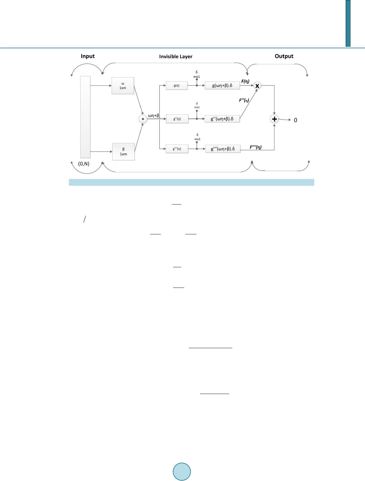

I. Ahmad, M. Bilal
225
Figure 1. Neural network architecture for Blasius equation.
2
2
d0 as
d
ux
x→ →∞
(4)
Put
xx η
∞
=
in Equations (1-3), we g e t
( )
32
32
dd
0; 01
dd
uu
xu
ηη
ηη
∞
+= <<
(5)
( )
00u=
(6)
d0 at 0
d
u
η
η
= =
(7)
2
2
d0 at 1
d
u
η
η
= =
(8)
We construct a mathematical model based on active set with fitness function. The system is based on
numerical computation through which we obtain optimum variables of the proposed model [11]-[13].
The solution
( )
u η
of the differential Equation (5) along with it’s derivatives, can be approximated by the
following continuous relations as in neural network methodology and the activation function Log-Sigmoid is
defined as
( )
1 exp
LS x
δ
βω
=+ −−
∑
(9)
Blasius equation mathematical mode l with the help of above activation function was developed to
approximate the solution of Equations (5-8) with
2
nd
and
3rd
order derivatives. Using this methodology the
solution
( )
u η
can be app roxima te d by
( )
( )
1
ˆ1e
mi
LS ii
i
u
β ωη
δ
η
−−
=
=+
∑
(10)
where
m
is the number of neurons,
δ
,
ω
, and
β
are real-valued bounded adaptive parameters or weights
can be expressed an array
W
as
( )
121 212
,,,,,,, ,,,,
mmm
W δδδ ωωω βββ = 
The second and third order derivatives of solution
( )
u η
can be approximation by the continuous relations

I. Ahmad, M. Bilal
226
( )
( )
( )
( )
()
( )
( )
( )
()
22
22
32
1
2e e
ˆ
1e 1e
i iii m
LSi i
iii ii
u
βωηβ ωη
βωη βωη
η δω
− −−−
−− −−
=


= −


++


∑
(11)
( )
( )
( )
( )
()
( )
( )
()
( )
( )
( )
()
33 22
33
43 2
1
6e 6ee
ˆ
1e 1e 1e
i iiiii
m
LSii
iii ii ii
u
βωηβωηβωη
βωη βωη βωη
η δω
− −− −−−
−− −− −−
=


= −+


+++


∑
(12)
where
( )
2
u
and
( )
3
u
represented
2nd
and
3rd
derivative with respect to
η
respectively.
The mathematical model for Equation (5) can be formulated by a linear combination of networks Equations
(10-12) is called a differential equation neural networks.
The fitness function for proposed model
∈
has been formulated for the Equations (5-8) using Mathematical
model by defining the error as the sum of mean squared errors:
123
∈=∈ +∈+∈
The error term
1
∈
is connected with the physical problem (5) with
1x
∞
=
is given as:
( )()
2
32
1
ˆˆˆ AVERAGE; for 1,1.
i ii
uuu iN

∈=+= +

(13)
where
( )
ˆ ˆ
ii
uu η =
, interval
[ ]
0,1
with step size
0.1 h=
is divided by
1N+
subintervals i.e.,
[ ] [] []
12 231
,, ,,,,
NN
ηηηηη η
+

.
And
2
∈
for initial values can be defined as
( )
( )
2
1
2 00
AVERAGE uu∈= +
(14)
For
1 η =
we have
( )
2
2
3
u

∈=
.
Optimization Procedure for Numerical Solution
Furthermore, we provide some detail about the procedural steps for the optimization in MATLAB built-in
function is given below.The generic flow diagram of the overall process is shown in Figure 2.
Step 1: Initialization:
A vector with randomly generated bounded real values of length equal to the number of weights in each
Mathematical model acts as the starting point for each solver:
( )
121 212
,,,,,,, ,,,
m mm
W δδδ ωωω βββ = 
Here m represents the number of neurons.
Step 2: Fitness Evaluation:
The MATLAB built-in function for constrained optimization problems is invoked for each model.
Step 3: Termination Criteria:
Terminate the execution of the solver, if any of the following criteria is satisfied:
•
required level of predefined fitness achieved, i.e.,
14
10
−
∈≤
.
•
total number of iterations executed, as listed in Table 1.
Step 4: Storage:
Save the final optimal weights (variables) along with fitness values and computational time taken by the
algorithm.
Step 5: Statistical Analysis :
Repeat steps 1 to 4 for sufficiently large number of times to perform an effective and reliable statistical
analysis.
4. Numerical Results
In this section, we show the output of the proposed method by the numerical results of Blasius equation. Further,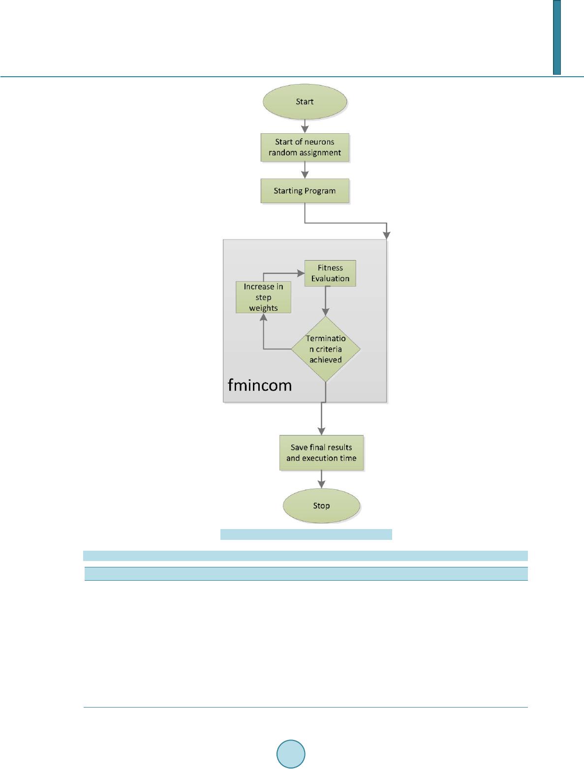

I. Ahmad, M. Bilal
227
Figure 2. Flow chart of Blasius equation model.
Table 1. Parameter settings for the function “fmincon” in MATLAB simulations.
Parameters Settings/Values
“Fin Diff Type” “Central”
Start Point generation Randomly between (0, 1)
Hessian BFGS
Minimum Perturbation
08
10−
Total Start Points
100
Max Iterations
1700
Max Fun Evals
1000000
Start Point Size
30 - 60
X Tolrence
14
10−
Scaling Objective and Constraints

I. Ahmad, M. Bilal
228
we calculate the values of
RF
u
called reference solution with MATHEMATICA, approximate solution
ˆLS
u
and the absolute error function
ˆ
RF LS
uu−
with hybrid AST-INP and SQP algorithms. Furthermore, we pro-
vided the statistical analysis with several time run of optimization tools for Mean, Median, STD and Variance
tabulated in Table 2 and Table 3 for both cases. Which showed that the present solution is highly accurate as
compared to others methods present in literature.
5. Statistical Analysis and Discussion
On the basis of the simulations and results obtained in the previous section, it can be concluded that Blasius
differential equation can be solved by stochastic computational intelligence technique, like SQP optimization
algorithm, AST-INP hybrid technique, supported with simulating annealing. The differential equation neural
networks trained by SQP algorithm and AST-INP are better stochastic optimizers as compared to other
algorithms. The statistical analysis f or this case with AST-INP and SQP algorithm are tabulated in Table 2 and
Table 3. These results showed the better accuracy of numerical data with reference solution. We presented
minimum value, mean, median and STD for the accuracy of our solver for 300 time multi-runs with minimum
time as shown in Table 2 and Table 3.
Table 2. Statistical analysis of solution of Blasius equation with hybrid (AST-INP).
η
Exact Mean Median STD Var
0 0 −8.24E−04 −5.79E−04 0.0017 2.98E−06
0.1 0.005215 0.0046 0.0047 0.0016 2.63E−06
0.2 0.020856 0.0204 0.0205 0.0016 2.58E−06
0.3 0.046911 0.0466 0.0466 0.0016 2.72E−06
0.4 0.083345 0.0832 0.0831 0.0017 2.95E−06
0.5 0.130089 0.13 0.1299 0.0018 3.21E−06
0.6 0.187034 0.1869 0.1868 0.0019 3.42E−06
0.7 0.254021 0.2539 0.2538 0.0019 3.57E−06
0.8 0.330829 0.3307 0.3306 0.0019 3.63E−06
0.9 0.417178 0.417 0.417 0.0019 3.61E−06
1 0.512716 0.5124 0.5124 0.0019 3.53E−06
Table 3. Statistical analysis of solution of Blasius equation with SQP.
η
Min Max Mean Median STD Var
0 −0.00546 0.00454 −0.00064 −0.00045 0.0013 1.66E−06
0.1 −9.03E−06 9.99E−03 4.68E−03 4.82E−03 0.0013 1.65E−06
0.2 0.01509 0.02587 0.0204 0.02055 0.0013 1.70E−06
0.3 0.04059 0.05216 0.04652 0.04665 0.0013 1.79E−06
0.4 0.07648 0.08881 0.083 0.08315 0.0014 1.91E−06
0.5 0.1227 0.1358 0.1298 0.1299 0.0014 2.04E−06
0.6 0.1791 0.1929 0.1867 0.1869 0.0015 2.18E−06
0.7 0.2456 0.26 0.2537 0.2539 0.0015 2.32E−06
0.8 0.322 0.3369 0.3305 0.3307 0.0016 2.44E−06
0.9 0.4079 0.4233 0.4168 0.417 0.0016 2.55E−06
1 0.5031 0.5189 0.5122 0.5125 0.0016 2.64E−06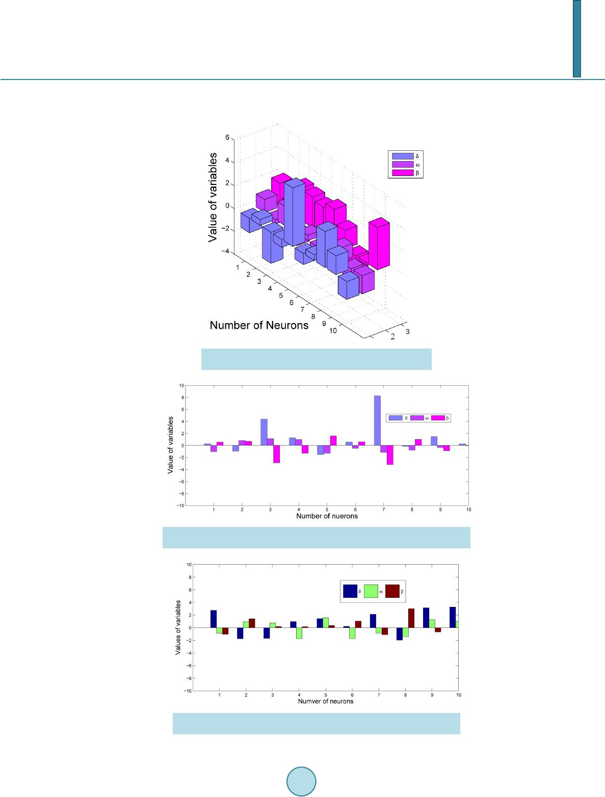

I. Ahmad, M. Bilal
229
Furthermore, Figure 3 and Figure 4 represented the 2-dimensional and 3-dimensional view of weights or
variables obtained from SQP optimizer. Similarly, Figure 5 and Figure 6 represented the 2-dimensional and
Figure 3. A 3D view of neural network model strained with
SQP for Blasius equation.
Figure 4. A 2D view of a set of variables of neural network model strained with
SQP for Blasius equation.
Figure 5. A 2D view of neural network model strained with hybrid (AST-INP)
for Blasius equation.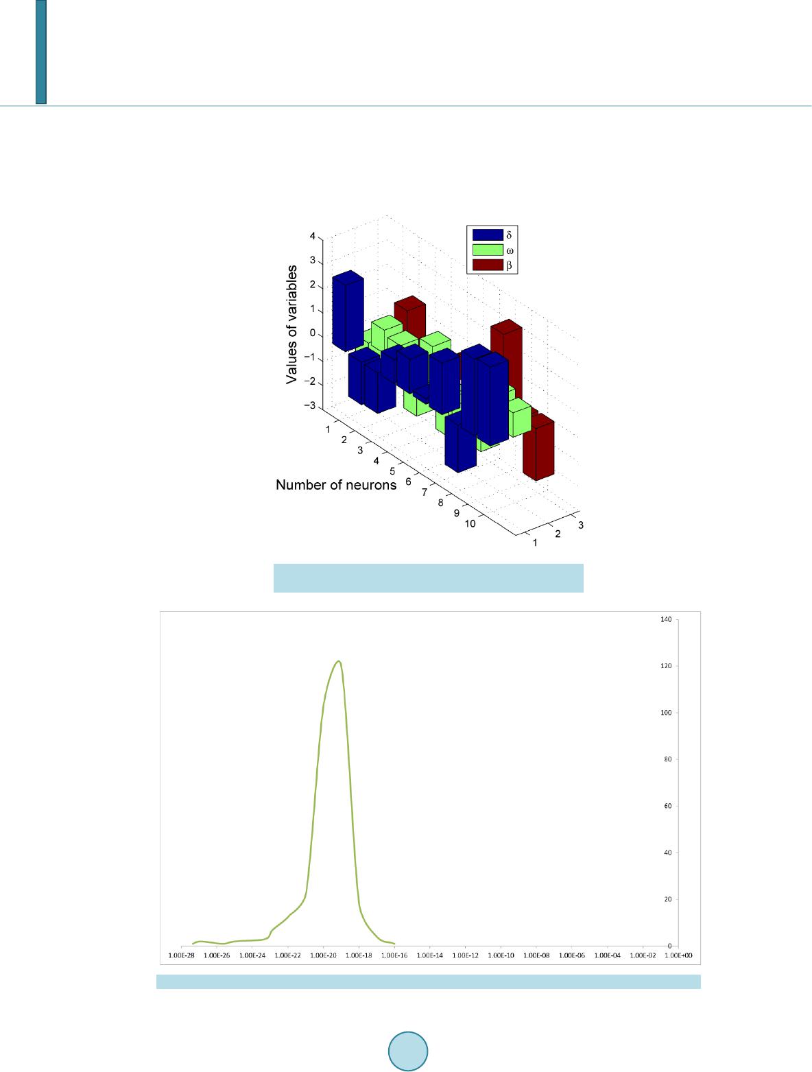

I. Ahmad, M. Bilal
230
3-dimensional view of weights or variables obtained from AST-INP optimizer. In Figure 7 , it is also shown that
the confidence level of absolute error at
20
10
−
is 90 percent and maximum values lies between
20
10
−
and
18
10
−
. We have shown the Chi-squares distribution fitness with normal form to the numerical data through
several time simulation as shown in Figure 8. Furthermore, in Figure 9, we presented the comparison of
reported results mean with exact solution (reference solution).
Figure 6. A 3D view of set of variables of neural network
model strained with hybrid (AST-INP) for Blasius equation.
Figure 7. Chi Square curve of 300 results shows the confidence level of our data.

I. Ahmad, M. Bilal
231
Figure 8. Fitness of Chi-square distribution with proposed data of Blasius
equation.
Figure 9. Mean V S Exact value of Blasius equation.
Thus it can be stated that proposed computing approach is reliable, effective and easily applicable for
complex differential equation of order three. In our future work, we intend to use other hybrid computational
intelligence algor ithms like GA-SQP, GA-INP and GA-AST to solve these problems using Bessel’s polynomial
as active function.
Acknowledgments
The author would like to thanks Dr Sirj-ul-Islam for help in this research work.
References
[1] Howarth, L. (1938) On the Solution of t he Laminar Boundary Layer Equations. Proc eedings of the London Mathemat-
ical Soc iety, 164, 547-579. http://dx.doi.org/10.1098/rspa.1938.0037
[2] Liao, S.J. (1999) An Explicit, T otally Analytic Approximate Solution for Blasius Viscous Flow Problems. Internation-
al Journal of Non-Linear Mechanics, 34, 759-778. http://dx.doi.org/10.1016/S0020-7462(98)00056-0

I. Ahmad, M. Bilal
232
[3] Liao, S.J. (1992) The Proposed Homotopy Analysis Technique for the Solution of Nonlinear Problems. Ph.D. Thesis,
Shanghai Jiao Tong University, Shanghai.
[4] Shishkin, G.I. (2001) Grid Approximation of the Solution to the Blasius Equation and of its Derivatives. Computation-
al Mathematics and Mathematical Physics, 41, 37-54.
[5] Yu, L.T. and Kuang, C.C. (1998) The Solution of the Blasius Equation by the Differential Transformation Method.
Mathematical and Computer Modeling, 28, 101-111.
[6] Schlichting, H. (1979) Boundary Layer Theory. McGraw-Hill, New York, 127-144.
[7] Coppel, W.A. (1960) On a Differential Equation of Boundary Layer Theory. Philosophical Transactions of the Royal
Society A, 253, 101-136.
[8] Allan, F.M. and Abu-Saris, R.M. (1999) On the Existence and Non-Uniqueness of Nonhomogeneous Blasius Problem.
Proceedings of the Second Pal. International Conference, Gorden and Breach, Newark.
[9] Howarth, L. (1938) On the Solution of t he Laminar Boundary Layer Equations. Proc eedings of the London Mathemat-
ical Soc iety, 164, 547-579. http://dx.doi.org/10.1098/rspa.1938.0037
[10] Liao, S.J. (1999) An Explicit, Totally Analytic Approximate Solution for Blasius Viscous Flow Problems. Internation-
al Journal of Non-Linear Mechanics, 34, 759-778. http://dx.doi.org/10.1016/S0020-7462(98)00056-0
[11] Khan, J.A. and Zahoor Raja, M.A. (2013) Artificial Intelligence based Solver for Governing Model of Radioactivity
Cooling, Self-Gravitating Clouds and Clusters of Galaxies. Research Journal of Applied Sciences, Engineering and
Technology, 6, 450-456.
[12] Zahoor Raja, M.A., Khan, J.A. and Qureshi, I.M. (2010) A New Stochastic Approach for Solution of Riccati Differen-
tial Equation of Fractional Order. Annals of Mathematics and Artificial Intelligence, 60, 229-250.
http://dx.doi.org/10.1007/s10472-010-9222-x
[13] Zahoor Raja, M.A. and Samar, R. (2014) Numerical Treatment for Nonlinear MHD Jeffery-Hamel Problem Using
Neural Networks Optimized with Interior Point Algorithm. Neurocomputing, 124, 178-193.
http://dx.doi.org/10.1016/j.neucom.2013.07.013