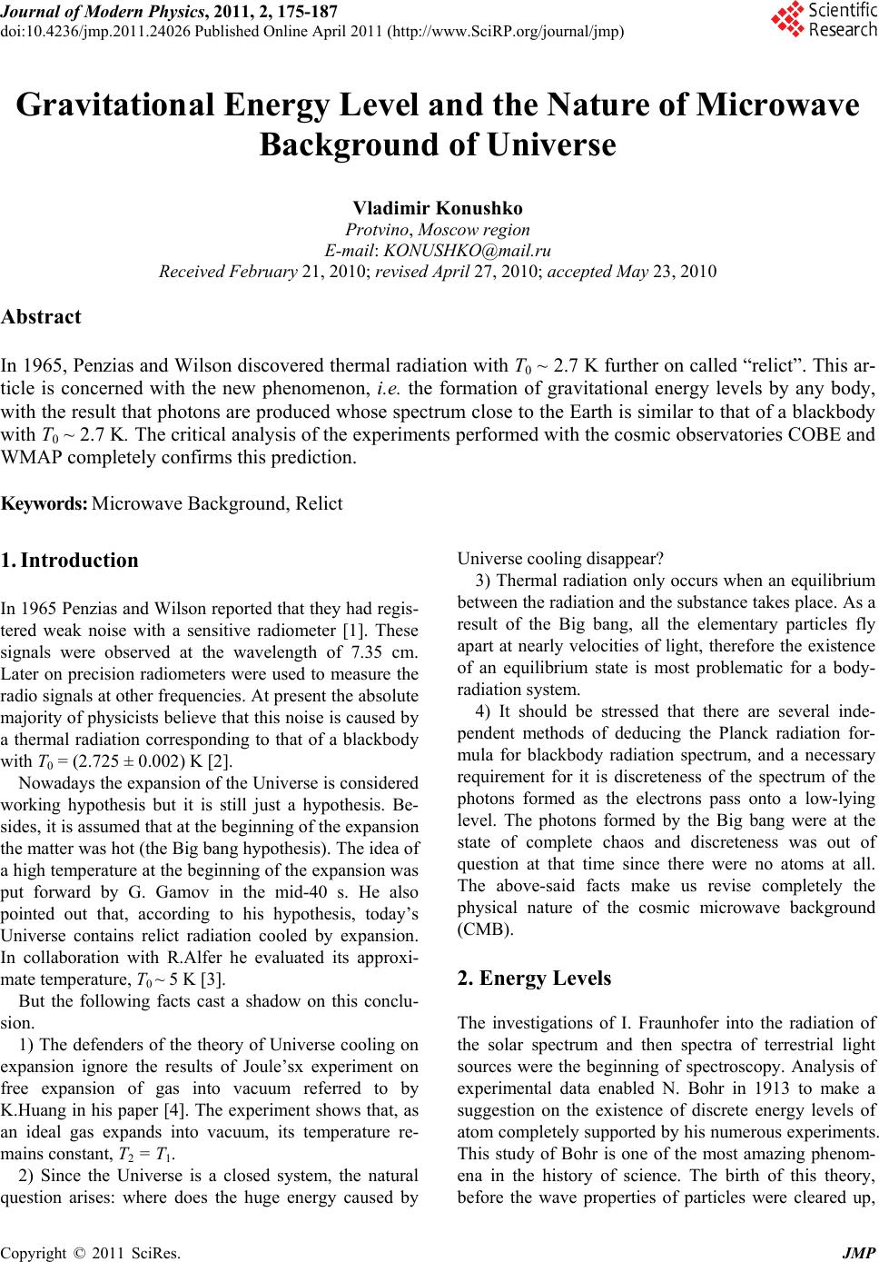Journal of Modern Physics, 2011, 2, 175-187
doi:10.4236/jmp.2011.24026 Published Online April 2011 (http://www.SciRP.org/journal/jmp)
175
Gravitational Energy Level and the Nature of Microwave
Background of Universe
Vladimir Konushko
Protvino, Moscow region
Received February 21 , 2010; revised April 27, 2010; accept e d May 23, 2010
Abstract
In 1965, Penzias and Wilson discovered thermal radiation with T0 ~ 2.7 K further on called “relict”. This ar-
ticle is concerned with the new phenomenon, i.e. the formation of gravitational energy levels by any body,
with the result that photons are produced whose spectrum close to the Earth is similar to that of a blackbody
with T0 ~ 2.7 K. The critical analysis of the experiments performed with the cosmic observatories COBE and
WMAP completely confirms this prediction.
Keywords: Microwave Background, Relict
1. Introduction
In 1965 Penzias and Wilson reported that they had regis-
tered weak noise with a sensitive radiometer [1]. These
signals were observed at the wavelength of 7.35 cm.
Later on precision radiometers were used to measure the
radio signals at other frequencies. At present the absolute
majority of physicists believ e that this noise is caused by
a thermal radiation corresponding to that of a blackbody
with T0 = (2.725 ± 0.002) K [2].
Nowadays the expansion of the Universe is considered
working hypothesis but it is still just a hypothesis. Be-
sides, it is assumed that at the beginning of the expansion
the matter was hot (the Big bang hypothesis). The idea of
a high temperature at the beginning of the expansion was
put forward by G. Gamov in the mid-40 s. He also
pointed out that, according to his hypothesis, today’s
Universe contains relict radiation cooled by expansion.
In collaboration with R.Alfer he evaluated its approxi-
mate temperature, T0 ~ 5 K [3].
But the following facts cast a shadow on this conclu-
sion.
1) The defenders of the theory of Universe cooling on
expansion ignore the results of Joule’sх experiment on
free expansion of gas into vacuum referred to by
K.Huang in his paper [4]. The experiment shows that, as
an ideal gas expands into vacuum, its temperature re-
mains constant, T2 = T1.
2) Since the Universe is a closed system, the natural
question arises: where does the huge energy caused by
Universe cooling disappear?
3) Thermal radiation only occurs when an equilibriu m
between the radiation and the substance takes place. As a
result of the Big bang, all the elementary particles fly
apart at nearly velocities of light, therefore the existence
of an equilibrium state is most problematic for a body-
radiation system.
4) It should be stressed that there are several inde-
pendent methods of deducing the Planck radiation for-
mula for blackbody radiation spectrum, and a necessary
requirement for it is discreteness of the spectrum of the
photons formed as the electrons pass onto a low-lying
level. The photons formed by the Big bang were at the
state of complete chaos and discreteness was out of
question at that time since there were no atoms at all.
The above-said facts make us revise completely the
physical nature of the cosmic microwave background
(CMB).
2. Energy Levels
The investigations of I. Fraunhofer into the radiation of
the solar spectrum and then spectra of terrestrial light
sources were the beginning of spectroscopy. Analysis of
experimental data enabled N. Bohr in 1913 to make a
suggestion on the existence of discrete energy levels of
atom completely supported by his numerous experiments.
This study of Bohr is one of the most amazing phenom-
ena in the history of science. The birth of this theory,
before the wave properties of particles were cleared up,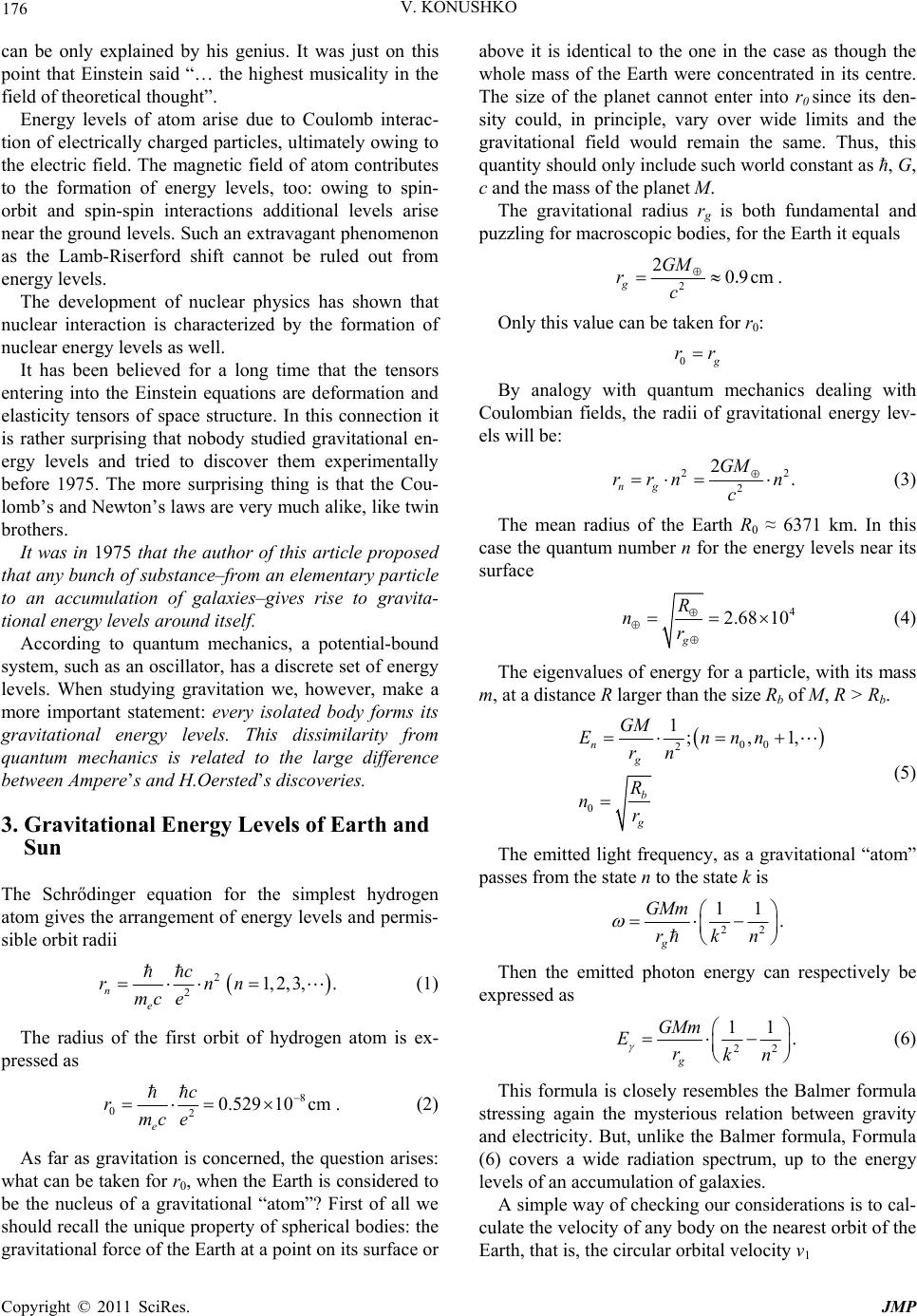

176 V. KONUSHKO
can be only explained by his genius. It was just on this
point that Einstein said “… the highest musicality in the
field of theoretical thought”.
Energy levels of atom arise due to Coulomb interac-
tion of electrically charged particles, ultimately owing to
the electric field. The magnetic field of atom contributes
to the formation of energy levels, too: owing to spin-
orbit and spin-spin interactions additional levels arise
near the ground levels. Such an extrav agant ph enomenon
as the Lamb-Riserford shift cannot be ruled out from
energy levels.
The development of nuclear physics has shown that
nuclear interaction is characterized by the formation of
nuclear energy levels as well.
It has been believed for a long time that the tensors
entering into the Einstein equations are deformation and
elasticity tensors of space structure. In this connection it
is rather surprising that nobody studied gravitational en-
ergy levels and tried to discover them experimentally
before 1975. The more surprising thing is that the Cou-
lomb’s and Newton’s laws are very much alike, like twin
brothers.
It was in 1975 that the author of this article proposed
that any bunch of substance–from an elementary particle
to an accumulation of galaxies–gives rise to gravita-
tional energy levels around itself.
According to quantum mechanics, a potential-bound
system, such as an oscillator, has a discrete set of energy
levels. When studying gravitation we, however, make a
more important statement: every isolated body forms its
gravitational energy levels. This dissimilarity from
quantum mechanics is related to the large difference
between Ampere’s and H. Oersted’s discoveries.
3. Gravitational Energy Levels of Earth and
Sun
The Schrődinger equation for the simplest hydrogen
atom gives the arrangement of energy levels and permis-
sible orbit radii

2
21, 2, 3,.
ne
c
rnn
mc e
 
 

(1)
The radius of the first orbit of hydrogen atom is ex-
pressed as
8
020.529 10cm
e
c
rmc e

 
 . (2)
As far as gravitation is concerned, the question arises:
what can be taken for r0, when th e Earth is con sidered to
be the nucleus of a gravitational “atom”? First of all we
should recall the unique property of spherical bodies: th e
gravitational force of the Earth at a point on its surface or
above it is identical to the one in the case as though the
whole mass of the Earth were concentrated in its centre.
The size of the planet cannot enter into r0 since its den-
sity could, in principle, vary over wide limits and the
gravitational field would remain the same. Thus, this
quantity should only in clud e such wo rld constan t as ћ, G,
c and the mass of the planet M.
The gravitational radius rg is both fundamental and
puzzling for macroscop ic bodies, for the Earth it equals
2
209cm
g
GM
rc

..
Only this value can be taken for r0:
0
g
rr
By analogy with quantum mechanics dealing with
Coulombian fields, the radii of gravitational energy lev-
els will be:
2
2
2.
ng
GM
rrn n
c
2

 (3)
The mean radius of the Earth R0 ≈ 6371 km. In this
case the quantum number n for the energy levels near its
surface
4
2.68 10
g
R
nr



 (4)
The eigenvalues of energy for a particle, with its mass
m, at a distan ce R larger than the size Rb of M, R > Rb.

00
2
0
1;,1,
ng
b
g
GM
Ennn
rn
R
nr
 


(5)
The emitted light frequency, as a gravitational “atom”
passes from the state n to the state k is
22
11
.
g
GMm
rkn






Then the emitted photon energy can respectively be
expressed as
22
11
.
g
GMm
Erkn







(6)
This formula is closely resembles the Balmer formula
stressing again the mysterious relation between gravity
and electricity. But, unlike the Balmer formula, Formula
(6) covers a wide radiation spectrum, up to the energy
levels of an accumulation of galaxies.
A simple way of ch ecking our cons iderations is to cal-
culate the velocity of any body on the nearest o rbit of the
Earth, that is, the circular orbital velocity ν1

V. KONUSHKO
177
3
1810msec
2
с
n



,
where c is the velocity at the first gravitational level n =
1, when r = rg, which means that c is the velocity of light
and we act by analogy with quantum mechanics. Thus,
the number = 2.68 × 104 is real and it confirms the
correctness of the choice r0 = rg.
n
The distance between two adjacent energy levels


1
21
nn
rr rnr


0
(7)
Near the Earth’s surface it equals
477 mr 
This value, which is small as compared to the radius of
the Eart h, shows that th e energy levels of such a gravita-
tional “atom” near the planet are so densely arranged that,
as electrons and protons pass onto a lower level the
quanta emitted form a continuous radiation spectrum. It
should be noted that the situation in atoms is quite dif-
ferent: the levels near the nucleus are very far-scattered.
But what kind of quanta are they? At first sight, as we
investigate gravity, they seem to be quanta of a gravita-
tional field, that is, gravitons.
And, nevertheless, electrons and protons are most
likely to emit photons and that is why. Any particle mov-
ing at a high speed cannot “remember” which physical
field–electronic, nonuniform magnetic or gravitational–
has transmitted energy to it. Hence, any energy levels
account for the deformation of space structure.
Leaving aside the very important problem of gravitons
for awhile, we shall go on studying the spectra of pho-
tons only emitted by the electrons passing from one
gravitational level of a macroscopic body (Earth, Sun,
stars) onto another one.
The quantum number n near the Sun’s surface
483
g
R
nr

.
In this case the distance between adjacent energy lev-
els nearly the Sun is
2900 kmr  .
This distance is extremely small, too, as compared to
the size of the Sun and, hence, its gravitational radiation
spectrum will be nearly continuous, too.
The basic decoration of the Saturn is its rings extend-
ing to about 60 000 km from the planet Figure 1.
The flights of space vehicles have shown that the rings
of the Saturn are not solid but consist of hundreds and
thousands of individual rings one inside the other and
separated by small “holes” of about 10 km. It is rather
interesting to calculate the distance between the gravita-
Figure 1. The fine structure of Saturn’s rings.
tional energy levels of this wonderful planet near its sur-
face using Formula (7) 14 kmr

.
No doubt, when observing the fine structure o f the Sat-
urn’s rings we can observe by the naked eye individual
gravitational energy levels.
Later ringed systems of small particles and bodies
were discovered around the Jupiter and the Uranus.
These systems resist usual observations from the Earth
but they have rather a complex structure.
Another surprising ability demonstrated by the Sun is
that the distance b etween the adjacent gravitational levels
formed by the Sun near the Earth’s surface will be
42100 kmr


This number astonishingly coincides with the distance
at which a geostationary sate like hanging over a certain
point of the Earth must revolve
2
3242100km
4
GMT
RH


 
,
where T is the period of revo lution of the planet, H is the
height over the Earth’s surface.
There is no question that the Earth is on a gravita-
tional level formed by the Sun. The short distances be-
tween adjacent energy levels near the surfaces of all the
planets in the solar system indicate that they are all the
positioned on energy levels. Hence we can make a very
important conclusion: just as electrons in atoms are
grouped on atomic energy levels, so cosmic dust and
fragments are grouped on the gravitational levels set up
by stars thus forming planets.
4. Gravitational Quasi-Blackbodied
Radiation
In the above parts we adduced convincing arguments in

178 V. KONUSHKO
favor of gravitational energy levels and now are going to
consider the sequences of this wonderful prediction. The
mean energy of black-bodied radiation with its frequency
ω can be expressed as
exp() 1kT

 

 (8)
Note that, with ћ tending to zero, Formula (8) changes
to the classical expression
kT   (9)
This can be supported by setting exp(ћω/kT) ≈ 1+
ћω/kT, which can be met the more precisely, the less ћ.
Thus, if the energy could assume a continuous series of
values, its mean value would be equal to kT.
As it has already been mentioned above, the gravita-
tional energy levels near both the Earth and the Sun and,
in general, nearby any body are arranged so densely that
the radiation spectrum produced by electrons, as they
pass from one gravitational level to another one, can be
considered continuous quasi-blackbodied.
As for the atomic structure, the radiation for far re-
moved orbits (that is, orbits more characterized by mac-
roscopic conditions) found by the use of the Bohr theory
as well as within the frameworks of quantum mechanics
approximates to the radiation found by the Maxwell the-
ory, that is, classical. For macroscopic bodies the quan-
tum number n is always large even near the surface (for
the Earth n = 26 800) thus complying with the classical
requirements. In the hydrogen atom the ground state is
characterized by the quantum number n = 1. That is why
we have kT in the right member of (9) but not 3/2kT.
It is known from thermodynamics that if a gas is in
equilibrium state (that is, in a state with constant pa-
rameters), the velocity distribution remains unchanged.
The electrons filling atoms the whole magnetosphere of
the Earth meet this requirement in a first approximation,
and one of the characteristics of this electron gas is the
mean kinetic energ y of electrons hitting the Earth.
From atomic physics it is evident that in excited atoms
the electrons on the higher energy levels tend to go back
to the nucleus if there are vacancies on the level n = 1.
In a similar manner, in the gravitational “atom” where
the nucleus is the Earth, the electrons at a large distance
from the Earth try to pass under gravity onto the level
closest to the planet and characterized by the circular
orbital velocity ν1. There can be no doubt that it is just
this velocity ν1 that is the most probable, νpr = ν1.
The energy conservation law for an electron on a
near-earth orbit takes the form:
2
1
2
ee
GM mm
R



,
hence,
2
1GM
R




The escape velocity ν2 is
2
22GM
R




When the elementary gas theory is applied to electrons,
the most probable velocity can be expressed as
22
pr e
kT
m
 
On the assumption ν1 = νpr we have
2
12
e
kT
m
 
The mean-square velocity of the electrons producing
electron gas will be:
28
e
kT
m
 
The relation between 2
1

and 2

becomes obvi-
ous
2
21
4

  
The mean kinetic energy takes the form
22
1
23
2e
mmGM
R






e
m
(10)
Using Formula (9) we get
2e GM mkT
R



 (11)
And, finally, the electron gas temperature near the
Earth can be found
22.64 K
e
GM m
TkR



 (12)
Since the spectrum of emitted p hotons faithfully copies
the spectrum of electrons, the above temperature can be
considered the temperature of quasi-black-bodied radia-
tion of the Ea rt h.
This temperature value is surprisingly close to that of
CMB measured by the Cosmic Background Explorer
(COBE) [2].
02.7250.002 KT

.
The whole ensuing material in this article will be suf-
ficient proof of the fact that the coincidence of these tem-
peratures is not accidental.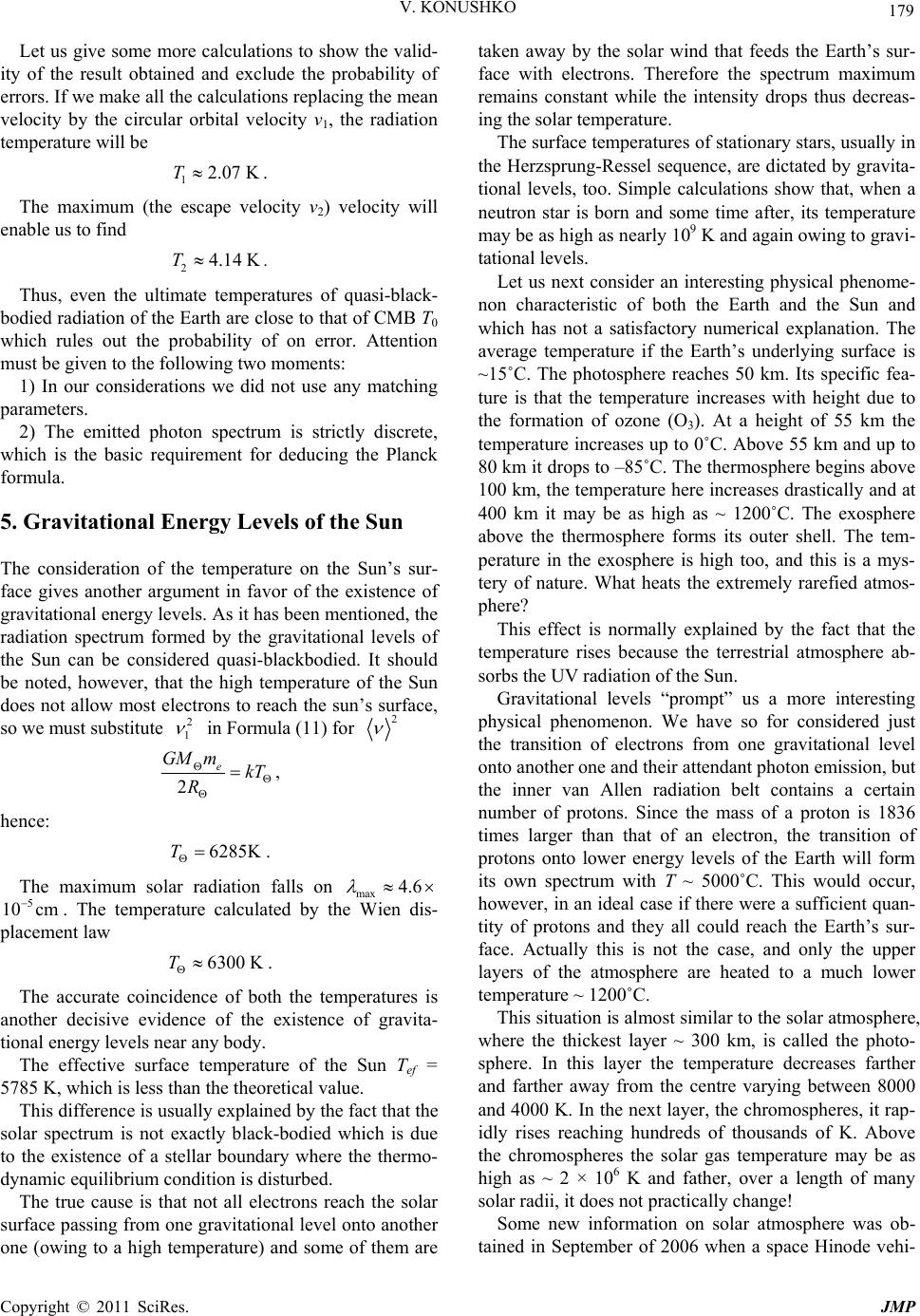

V. KONUSHKO
179
Let us give some more calculations to show the valid-
ity of the result obtained and exclude the probability of
errors. If we make all the calculations replacing the mean
velocity by the circular orbital velocity ν1, the radiation
temperature will be
12.07 KT.
The maximum (the escape velocity ν2) velocity will
enable us to find
24.14KT.
Thus, even the ultimate temperatures of quasi-black-
bodied radiation of the Earth are close to that of CMB T0
which rules out the probability of on error. Attention
must be given to the following two moments:
1) In our considerations we did not use any matching
parameters.
2) The emitted photon spectrum is strictly discrete,
which is the basic requirement for deducing the Planck
formula.
5. Gravitational Energy Levels of the Sun
The consideration of the temperature on the Sun’s sur-
face gives another argument in favor of the existence of
gravitational energy levels. As it has been mentioned, the
radiation spectrum formed by the gravitational levels of
the Sun can be considered quasi-blackbodied. It should
be noted, however, that the high temperature of the Sun
does not allow most electrons to reach the sun’s surface,
so we must substitute 2
1

in Formula (11) for 2

2e
GM mkT
R


,
hence:
6285KT.
The maximum solar radiation falls on max 4.6



. The temperature calculated by the Wien dis-
placement law
5
10 cm

6300 KT.
The accurate coincidence of both the temperatures is
another decisive evidence of the existence of gravita-
tional energy levels near any body.
The effective surface temperature of the Sun Tef =
5785 K, which is less than the theoretical value.
This difference is usually explained by the fact that the
solar spectrum is not exactly black-bodied which is due
to the existence of a stellar boundary where the thermo-
dynamic equilibrium condition is disturbed.
The true cause is that not all electrons reach the solar
surface passing from one gravitational level onto another
one (owing to a high temperature) and some of them are
taken away by the solar wind that feeds the Earth’s sur-
face with electrons. Therefore the spectrum maximum
remains constant while the intensity drops thus decreas-
ing the solar temperature.
The surface temperatures of stationary stars, usually in
the Herzsprung-Ressel sequence, are dictated by gravita-
tional levels, too. Simple calculations show that, when a
neutron star is born and some time after, its temperature
may be as high as nearly 109 K and again owing to gravi-
tational levels.
Let us next consider an interesting physical phenome-
non characteristic of both the Earth and the Sun and
which has not a satisfactory numerical explanation. The
average temperature if the Earth’s underlying surface is
~15˚C. The photosphere reaches 50 km. Its specific fea-
ture is that the temperature increases with height due to
the formation of ozone (O3). At a height of 55 km the
temperature increases up to 0˚C. Above 55 km and up to
80 km it drops to –85˚C. The thermosphere begins above
100 km, the temperature here increases drastically and at
400 km it may be as high as ~ 1200˚C. The exosphere
above the thermosphere forms its outer shell. The tem-
perature in the exosphere is high too, and this is a mys-
tery of nature. What heats the extremely rarefied atmos-
phere?
This effect is normally explained by the fact that the
temperature rises because the terrestrial atmosphere ab-
sorbs the UV radiation of the Sun.
Gravitational levels “prompt” us a more interesting
physical phenomenon. We have so for considered just
the transition of electrons from one gravitational level
onto another one and their attendant photon emission, but
the inner van Allen radiation belt contains a certain
number of protons. Since the mass of a proton is 1836
times larger than that of an electron, the transition of
protons onto lower energy levels of the Earth will form
its own spectrum with T ~ 5000˚C. This would occur,
however, in an ideal case if there were a sufficient quan-
tity of protons and they all could reach the Earth’s sur-
face. Actually this is not the case, and only the upper
layers of the atmosphere are heated to a much lower
temperature ~ 1200˚C.
This situation is almost similar to the solar atmosphere,
where the thickest layer ~ 300 km, is called the photo-
sphere. In this layer the temperature decreases farther
and farther away from the centre varying between 8000
and 4000 K. In the next layer, the chromosph eres, it rap-
idly rises reaching hundreds of thousands of K. Above
the chromospheres the solar gas temperature may be as
high as ~ 2 × 106 K and father, over a length of many
solar radii, it does not practically change!
Some new information on solar atmosphere was ob-
tained in September of 2006 when a space Hinode vehi-

180 V. KONUSHKO
cle was launched. This information co rroborates fully the
abnormally high temperature of the solar corona-over
2 000 000 K.
The heating of the upper layers of the solar atmos-
phere is traditionally believed to be caused by the wave
motion of substance arising in the convectional zone.
These waves pass through the photosphere and carry into
the chromospheres and the corona a small fraction of the
mechanical energy which the gases in the convectional
zone possess.
But the outer surface of the photosphere has a tem-
perature just ~ 4000 K and the above explanation does
not stand up.
Let’s turn our attention to the gravitational levels of
the Sun again. The temperature, which would be set up
as a result of proton emission on the energy levels on the
solar surface, would reach ~11 × 106 K. This value is
nearly equal to the temperature of the solar core where
thermonuclea r reacti ons proceed.
We shall have a more striking result if we consider the
initial period when the incipient Sun can be considered
cold and we have to use a2

instead of 2
1

in tem-
perature calculations.
22
1
8
2

 

.
The solar surface temperature in this case may be as
high as 14 × 10 6 K (when thermonuclear reactions start).
Consequently, gravitational energy levels can be a match
that lights stars.
And again the deficient number of free protons (a part
of them fly away into word space in the form of a solar
wind) and the high solar surface temperature, at which
highly excited atoms can emit, allow the effect under
consideration to heat just the upper layers of the solar
atmospher e up t o 2 × 106 K.
6. The Fine Structure of the Earth’s
Gravitational Potential and Its
Consequences
The temperature (T ≈ 2.64 K) of the microwave back-
ground set up by the Earth has been obtained by us as-
suming that the planet is shaped lik e an ideal b all with its
radius .
6371kmR
But the Earth’s surface is described in fact by an indi-
vidual figure called a geoid [5].
The difference between the surface of a geoid and an
ellipsoid (spheroid) does not exceed several tens of me-
ters, whereas the difference between the equatorial and
the polar radii (Re and Rp) comes to 21.385 km. The ge-
oid oblateness a equal to
10.0033
298.255
ep
e
RR
aR

  .
According to Newton’s law, the attraction of a unit
mass by an element of mass dm at a distance r can be
expressed as
2
Gdm
Fr ,
where G is the gravitational constant. The potential of
attraction by a body at a point out side it in this case will
be
dm
UGr . (13)
The solution of the equation presen ts an infinite series
the coefficients of which are Legendre polynomials


cos
n
P

, which arise in our consideration in a natural
way. The first correction term for Equation (13) was de-
termined even before launching artificial Earth satellites
by means of ground measurements [5].

22
1c
e
GM R
UIP
RR os







 


, (14)
where I2 is the quadrupole amplitude the analogue of
which in the WMAP experiment [2] is the CMB anisot-
ropy amplitude C1.
The value of I2 is equal to 1082.65 × 10–6 which
causes the quadrupole expansion term to contribute to
the CMB temperature
22
3mKTTUIT

 .
This value remarkably coincides with that of the di-
pole amplitude l = 1 measured by the COBE [2]


13.3530.024 mKT 
This result was adjusted by the WMAP


13.3460.017 mKT 
A very important fact for us is that the WMAP did not
directly measure the dipole but obtained this value by
determining the residual dipole in processing.
The quadrupole l = 2 measured by the WMAP has a
very low amplitude


22
2154 70KT


or


212.5 8.5KT

.
To understand the situation involving the quadrupole
we should point up to the following.
The multipole expansion of the gravitational potential
allowed finding the contribution of the quadrupole ≈ 3

V. KONUSHKO
181
mK to the temperature T0 of micro wav e b a ck gro und . Th e
WMAP, however, determined the anisotropy of quadru-
pole rather then the temperature or the gradient of quad-
rupole. We should stress again that the difference in
height between a genoid and a spheroid does not exceed
a2 × R ≈ 70 m which makes up a negligible quantity ~
1.1 × 10–5. It is this fact that explains the large difference
between the negligible ∆T2 measu red by the WMAP and
the one predicted by the inflation hypothesis.
In its turn, this means that a large accumulation of gal-
axies referred to as the local Superaccumulation moves
at a velocity ~ 600 km/sec about the background. It has
been believed so far that the centre of this mass must
most likely be on rest about the whole distribution of
galaxies in the Universe and, hence, about the “relict”
background. If the COBE measures the contribution of
not the dipole but the quadrupole of the Earth’s gravita-
tional field, this treatment no longer arises and the local
Superaccumulation is really on rest. We have to suggest that the COBE measured not the
dipole but the contribution of the quadrupole to the
Earth’s gravitational potential since, besides rather
faithful coincidence of the numerical values, there is an-
other surprising agreement.
The measurements yielded sensationally small back-
ground anisotropy amplitudes with small ℓ: C2, C3, C4,
C5 [2]


2,3,4,530 KT



Quite are army of astrophysicists analyze the WMAP
results (we mainly refer to [6-8]) and some teams dis-
covered nearly a complete coincidence in dipole and
quadrupole principal axes which fully disagrees with the
predicting of the inflation hypothesis.
It should be stressed they are small within the frame-
works of the inflation hypothesis. And what did the
measurements of the Earth’s gravitatio nal potential give?
The expression for the U potential in the presence of
hydrostatic equilibrium (there is only pressure present
and tangential voltages are absent) must contain only
even moments I2n which decrease in magnitude with in-
creasing n:
If we share the opinion of most of the astrophysicists,
the COBE measurements of the dipole amplitude C1 are
directly related to the motion of the Earth abou t the CMB
with ν ≈ 390 ± 60 km/sec towards the Lion constellation .
  
221
1cos coscos
nn
nm
ee
nnn nmnm
nnm
RR
GM
UIP PAmB
RR Rsinm





 
 

 
 




where Anm, Bnm are gravitational moments determin ed by
experiments.
The measurements by artificial satellites, however,
gave a sensational result, too: all the gravitational mo-
ments starting with I3 are approximately of the same or-
der ~ 10–6 - 10–5. The decrease of moments with increas-
ing n in this case occurs much slower than has been sus-
pected. This, in its turn, leads to small temperature mul-
tifields

2,3,4,530 K,T 

which completely agrees with experiment [2] (Figure 2).
Note that the ordinate in the diagram is
2
1
T
Figure two shows experimental data without error. For
comparison, the results of the first year of WMAP opera-
tion are given with measurement errors (Figure 3)
Here we can see again a surprising agreement between
the experimental data obtained by COBE and WMAP
measurements and the results of harmonic analysis of the
gravitational potential:
Tө ~ 2,7 K T
g ~ 2,7 K
ΔT1 ~ 3 MK ΔT2 ~ 3 mK
T2 ~ 10 µK ΔT3 ~ 10 µK
ΔT(ℓ = 3,4,,20) ~ 30 µK ΔT(ℓ = 4,,10) ~ 30 µK
The supporters of the inflation hypothesis draw far
reaching conclusions observing ups and downs in the
angular power spectrum. We cannot produce this dia-
gram since there are restrictions on the harmonic analysis
of gravitational multipoles, ℓ ≤ 10, in view of practical
needs.
We are not doubted, however, that if gravitational
measurements were performed on a large scale and har-
monic analysis was made up to ℓ = 1000, we would be
bound to produce an oscillating curve for the following
reason. As the oblate ness of the Earth a ~ 1/300 and the
gravitational anomalies are very small and a fine ani-
sotropy structure can only be observed just with Θ ≤ 1˚;
at large angles the pattern spreads much like in experi-
ments of photon scattering on two slits the diffraction
pattern (fine structure) can only be observed when the
light wavelength λ is smaller than the distance between
the slits d. If λ < d, the diffraction pattern disappears.
The geoid heights are proportional to the amplitude of
gravitational anomalies. It is rather surprising that the
anomalies are not related to the topographic peculiarities
of the Earth (mountains, depressions, seas, etc.); the
presence of mountains almost does not affect gravimetric
measurements. Gravity anomalies are caused by some
density fluctuations in the Earth’s crust and mantle, are
very small in size (a2R ~ 70 m) and so the temperature

182 V. KONUSHKO
Figure 2. Temperature anisotropy within the frameworks
of multipole analysis after the first year of WMAP opera-
tion compared with other experiments.
Figure 3. Temperature anisotropy after the first year of
WMAP operation.
fluctuations separated by large angles are not related at
all.
The above-said is concerned with the C(Θ) function
(Figure 4).
The effect of amplitude smallness with small ℓ man i-
fests itself still stronger if we consider the angular corre-
lation function C(Θ) (Figure 4) instead of spherical
function Cℓ. The C(Θ) function denotes the correlation
degree of temperature fluctuations, an average value for
various pairs of dots in the sky separated by an angle Θ.
 
121 cos
4
CC

P

 

.
The observations [2] show that C(Θ) is almost equal to
zero for angles over 60˚; are not related at all.
The absence of wide-angle correlations was first ob-
served by the COBE and now has been confirmed by the
WMAP. The smallness of C(Θ) for wide angles means
not only that C2 and C3 are small but also that the ratio
between the first several amplitudes, at least up to C4, is
Figure 4. The correlation function of CMB temperature
measured by WMAP and COBE [2].
abnormal too. It should be noted again that a weak
power spectrum at wide angles is in a striking contradic-
tion with all the classical inflation models and can be
fully explained by the fact that the gravitational anoma-
lies of the Earth are extremely small.
7. Orientation of Multipoles (Experiment)
The results of studies into the orientation of many mul-
tipoles have become a real sensation bordering mysti-
cism. When dealing with this problem we should refer to
[6-8].
1) In 2003 Angelica de Oliveira-Costa and Max Teg-
mark from Pennsylvania University, Matias Zaldarriuga
from Colorado University in Boulder discovered that the
main axes of the quadrupole (ℓ = 2) and octupole (ℓ = 3)
modes are directed closely to each other and have a defi-
cient amplitude. But most of the inflation models suggest
that there should not be anything common between these
modes.
2) In the same year Hans Christian Eriksen and his
colleagues from Norway University in Oslo revealed a
coincidence in directions [7]. They divided the sky into
various pairs of hemispheres and evaluated the relative
amplitude fluctuations on the opposite halves of the sky.
The results of their investigation were fully inconsistent
with standard inflation cosmology: many pairs of hemi-
spheres differed considerab ly in power spectrum. But the
most unexpected thing is that a pain of the most different
hemispheres is evenly divided by an ecliptic, that is, by
the plane in which the orbit of motion of the Earth
around the Sun lies! (Figure 5).
Besides the too low amplitude with small ℓ, three more
dots can be observed (ℓ = 22, ℓ = 40 and ℓ = 210) (Fig-
ure 2) where the power spectrum considerably differs
from the one predicted by inflation models. Despite the
fact that these distinctions had been widely known, most
of the cosmologists missed the fact that the three devia-
tions correlated with th e eclectic, too.

V. KONUSHKO
183
–
80 μK 80 μK
Figure 5. The plane of ecliptic (dashed line) divides the full
sky map into a cold and a hot part. The northern part of
the ecliptic hemisphere is much colder than the southern
one. Account is taken of the contribution of only the quad-
rupole and the octupole to microwave background anisot-
ropy; the same can be observed in case of higher multipoles
as well.
3) In 2004 Domenic J. Schwarz, Glenn Starkman with
Craig Copi and Dragan Huterer from the University
Cleveland, Ohio, developed a new method of presenting
the “relict” background fluctuations in a vector form [8].
This enabled them to verify the speculation that the mi-
crowave background fluctuations must not be related to
special directions in the Universe.
Also, these scientists discovered unexpected correla-
tions supporting the results obtained by Oliveira Costa
and her colleagues [6].
The quadrupole (ℓ = 2, blue dots – 2) and the octupole
(ℓ = 3, red dots – 1) must be random oriented but, instead,
they tend to the equinox dots (hollow circles – 4) and
towards the motion of the solar system defined by the
dipole axis (ℓ = 1, green dots – 3) (Figure 6).
Moreover, their axes lie in the plane of ecliptic (v iolet
line – 5). Two of them (ℓ = 3, red dots – 1) are in the
plane of Supergalaxy, that is, the Local Superaccumula-
tion combining our Galaxy, its adjacent star systems and
their accumulations (orange line – 6). The probability of
random coincidence of these directions is < 10–4 (without
regard for the strange properties of low-order multiplets).
The agreement of the dipole and quadrupole axes re-
ferred to before and now may have resulted in the situa-
tion when the COBE measured the contribution of the
gravitational quadrupole (rather than its anisotropy) to
the microwave background as it has been mentioned
above.
The adherents of “relict” radiation, and they make up
the absolute majority, tried to explain the correlation
between low modes and the solar system structure by one
of the three methods.
First, an error in design of WMAP instruments or
wrong analysis of the data obtained (a systematic error).
But the WMAP team were rather careful and performed
Figure 6. The orientation of the first tree multipoles.
a lot of cross-tests for their instruments. So it is difficult
to imagine how the long correlations cou ld arise. Besides,
the authors [6-8] disclosed similar correlations in the
maps obtained by the COBE that made use of quite dif-
ferent instruments and analysis techniques.
The second explanation shows that there exists an un-
accounted source or absorber of microwave photons re-
lated to the solar system, for example, an unknown dust
cloud on its periphery. But how did this source or ab-
sorber of radiation happen to be observed by instruments
emitting microwave radiation but was not detected by
other numerous astronomical instruments over different
wavelength ranges?
At first sight, a discovery of local distortion of micro-
wave background data could solve the problem of its
large-scale fluctuations being weak. What actually hap-
pens is that it just makes the problem more complicated.
With the contribution to radiation associated with hypo-
thetic foreground objects subtracted, the residual cosmo-
logical contribution will be much smaller than consid-
ered before (any other conclusion would call for a ran-
dom but exact compensation between the cosmological
contribution and the predicted foreground source). In this
case it would be much more difficult to assert that the
absence of modes with small ℓ in the power spectrum is
just freak of chance.
And, finally, the third attempt to explain only the ab-
sence of modes with small ℓ in the power spectrum is
connected with topology since it has been impossible so
far to invent a physical mechanism for their suppression.
It is evident that these atte mpts cannot satisfy us because
they are ad hoc hypotheses in the proper sense of this
word.
8. Orientation of Gravitational Mult i po le s
To understand all the surprises connected with the mi-
crowave background we should again consider such a
fundamental physical phenomenon as the gravitational
energy levels formed by the Earth.
As it has already been mentioned several times, the

184 V. KONUSHKO
shape of the Earth just slightly differs from a sphere, its
oblate ness a ~ 1/300, and the South pole is only 30 m
closer to the centre of the Earth than the North pole.
When expanding a gravitational potential in terms of
Legandre polynoms we only apply one spherical coordi-
nate system (R, Θ, λ) and, hence, the directions of the
principle axes of a quadrupole, octupole and other
higher multipoles theoretically agree, and the Earth’s
symmetrical and equilibrium shape “confirms” this
agreement.
One of the significant discoveries of the present time
is spotting extremely intense radiation at distances of up
to several Earth’s radii [5]. The intensity of this rad iation
is millions of times higher than that of the cosmic rays
observed until recently in the terrestrial atmosphere.
Later on, the zones, where particles captured by the
geomagnetic field are concentrated, were given the name
radiation belts. Low-energy electrons fill almost the
whole magnetic sphere of the Earth. The outer boundary
of the magnetic sphere is at a distance r ≥ 10 R

. A little
the studies into radiation detected a new physical phe-
nomenon predicted by E. Parker: an ionized gas flow,
referred to as the solar wind, travels from the Sun at a
velocity ~ 400-600 km/sec and replenishes steadily the
number of charged particles in the Earth atmosphere. At
calm periods the intensity of electrons may be as high as
J ~ 108 cm–2·sec–1 and their spatial concentration varies
between several particles and several tens per 1 cm3.
During magnetic radiations their variation comes to two
orders. The inner part of the magnetic sphere lying a di-
pole-like geomagnetic field (up to 3) is referred to as
the plasma sphere. The concentration of “cold plasma”
particles in the plasma sphere is ~104cm–.
R
Hence, around the Earth there is a sufficient quantity
of electrons whose transition from one gravitational en-
ergy level onto a lower-lying level is followed by emis-
sion of low-energy photons forming quasi-black-bodied
radiation – CMB. The number of microwave background
photons in a uni t volume must be n ~ 410.
The electric charge of the Earth in this case does not
increase since the emitted electrons pass again onto
higher-lying levels (the Earth’s temperature is ~280 K)
and the whole process of radiation reminds a process
with any black body. The only difference is that the lev-
els are gravitational now rather than Coulomb-like.
Since the Sun is the only main supplier of electrons
onto the Earth, the CMB spectrum reflects this depend-
ence, an ecliptic dependence.
Another source of particles may be the ionized shell
round the Sun where the electron energy comes to just
several electron-volts.
Electron trapping has an interesting feature: the field
of trapping differs on the night and the day sides of the
Earth. On the day side it spreads almost to the boundar ies
of the magnetic sphere whereas on the night side it takes
just a small part of the latter.
This effect manifests itself particularly strongly at the
moment when the Earth is at the equitoctial points, that
is, when the day is equal to the night. That is why the
dependence of the CMB spectrum on the equitoctial
points is so mysterious.
It should be said finally how the two octupole axes (ℓ =
3) have been brought into the Supergalaxy plane. It is
well known that the velocity of the Galaxy about the
Supergalaxy is estimated at 400-500 km/sec. But, strange
as it may seem, this velocity is directed at an angle ≈
120˚ to, as it is widely believed, the direction of the
Earth’s motion relative to the CMB determined by the
dipole axis. But, as it has been mentioned, the dipole
axes almost coincide with the quadrupole and the octu-
pole axes (Figure 6). The angle between the octupole
axes, in its turn, is 60˚. So it is not surprising that a pair
of octupole axes lies in the Supergalaxy plane.
9. Microwave Background Polarization
It is well known that the Earth has a magnetic field. The
geomagnetic field induction B differs in magnitude and
direction at different points of the Earth’s surface. Be-
sides, the geomagnetic field elements remain constant in
time but all the time change their values.
The fact that the Earth has a magnetic field is respon-
sible for partial polarization of such elementary particles
as electrons, protons and neutron near the planet. This
polarization depends on the place and the time of obser-
vation, that is, it fluctuates strongly. When passing from
one gravitational level onto another one electrons and
protons emit photons which get partially polarized thanks
to their parents, and this polarization will fluctuate, too.
The solar plasma (solar wind) collid ing with the mag-
netic sphere of the Earth begin to flow around it. The
positive particles in this ca se are deflected eastward and
the negative particles westward. The flow is subjected to
polarization which can be described by an equivalent
current J counter-clockwise directed as viewed from the
North Pole. The new WMAP information [9] gives stun-
ning verification of this surprising polarization directiv-
ity of the photons emitted by polarized electro ns (Figure
7) partial polarization to the “relict” radiation generated
during recombination is in doubt since over the period
elapsed, 13 × 109 years, this partial polarization should
have died away inevitably because of multiple elastic
scattering.
In a first approximation the geomagnetic field is pre-
sented by a magnetic dipole at ~ 340 km from the centre
of the Earth. The investigations performed by Earth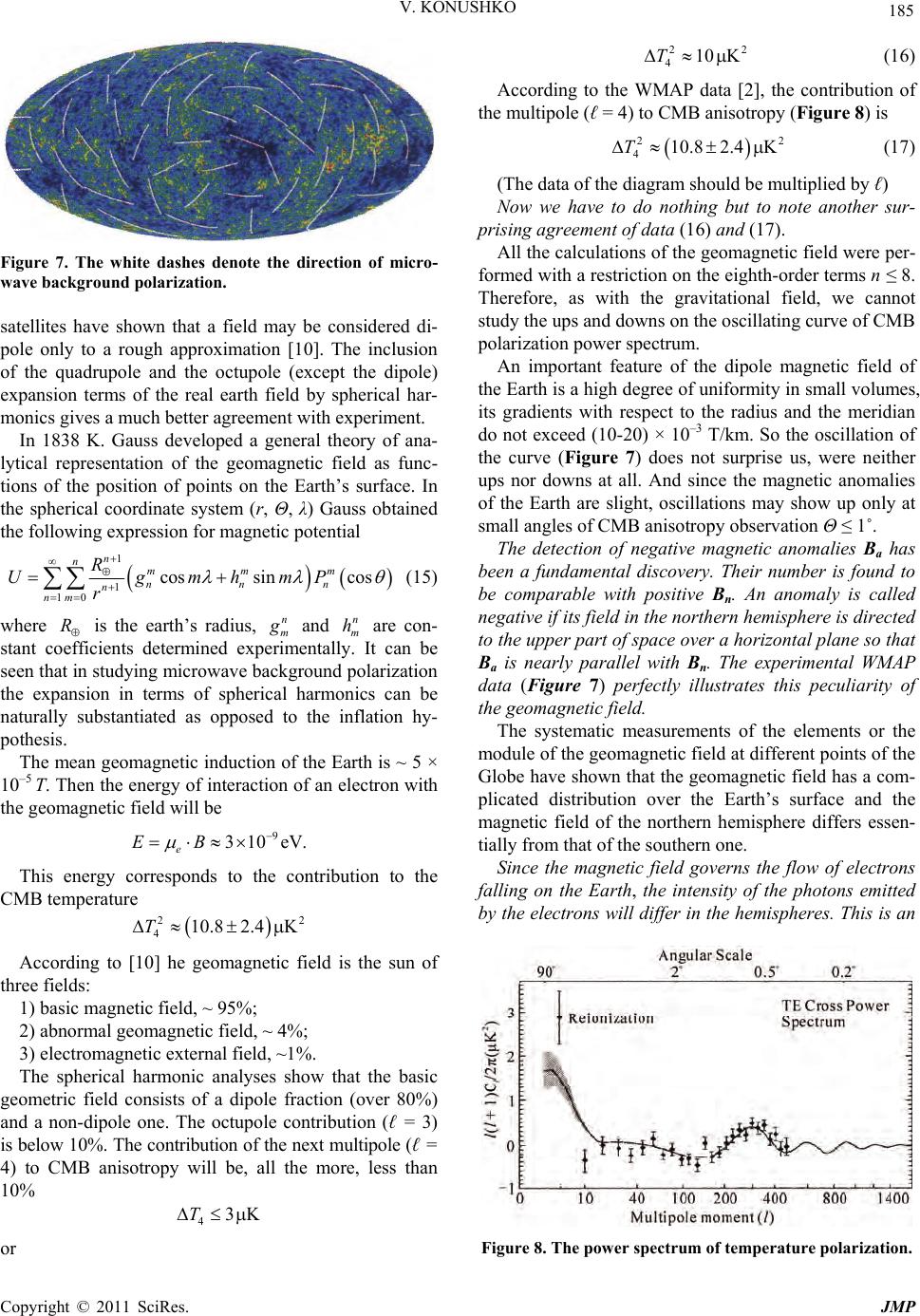

V. KONUSHKO
185
Figure 7. The white dashes denote the direction of micro-
wave background polarization.
satellites have shown that a field may be considered di-
pole only to a rough approximation [10]. The inclusion
of the quadrupole and the octupole (except the dipole)
expansion terms of the real earth field by spherical har-
monics gives a much better agreement with experiment.
In 1838 K. Gauss developed a general theory of ana-
lytical representation of the geomagnetic field as func-
tions of the position of points on the Earth’s surface. In
the spherical coordinate system (r, Θ, λ) Gauss obtained
the following expression for magnetic potential


1
1
10 cos sincos
n
nmmm
nnn
n
nm
R
UgmhmP
r









 (15)
where is the earth’s radius, Rn
m
g
and are con-
stant coefficients determined experimentally. It can be
seen that in studying microwave backgro und polarization
the expansion in terms of spherical harmonics can be
naturally substantiated as opposed to the inflation hy-
pothesis.
n
m
h
The mean geomagnetic induction of the Earth is ~ 5 ×
10–5 T. Then the energy of interaction of an electron with
the geomagnetic field will be
9
310eV.
e
EB 


This energy corresponds to the contribution to the
CMB temperature

22
410.8 2.4KT
According to [10] he geomagnetic field is the sun of
three fields:
1) basic magnetic field, ~ 95%;
2) abnormal geomagnetic field, ~ 4%;
3) electromagnetic external field, ~1%.
The spherical harmonic analyses show that the basic
geometric field consists of a dipole fraction (over 80%)
and a non-dipole one. The octupole contribution (ℓ = 3)
is below 10%. The contribution of the next multipole (ℓ =
4) to CMB anisotropy will be, all the more, less than
10%
43KT
or
2
410 KT2

 (16)
According to the WMAP data [2], the contribution of
the multipole (ℓ = 4) to CMB anisotropy (Figure 8) is


2
410.8 2.4KT2

 (17)
(The data of the diagram should be multiplied by ℓ)
Now we have to do nothing but to note another sur-
prising agreement of d ata (16) and (17).
All the calculations of the geomagnetic field were per-
formed with a restriction on the eighth-order terms n ≤ 8.
Therefore, as with the gravitational field, we cannot
study the ups and down s on th e oscillatin g cu rv e of CMB
polarization power spectrum.
An important feature of the dipole magnetic field of
the Earth is a high degree of unifor mity in small volumes,
its gradients with respect to the radius and the meridian
do not exceed (10-20) × 10–3 T/km. So the oscillation of
the curve (Figure 7) does not surprise us, were neither
ups nor downs at all. And since the magnetic anomalies
of the Earth are slight, oscillations may show up only at
small angles of CMB anisotropy observation Θ ≤ 1˚.
The detection of negative magnetic anomalies Ba has
been a fundamental discovery. Their number is found to
be comparable with positive Bn. An anomaly is called
negative if its field in the north ern hemisphere is directed
to the upper part of space over a horizontal plane so that
Ba is nearly parallel with Bn. The experimental WMAP
data (Figure 7) perfectly illustrates this peculiarity of
the geomagnetic field.
The systematic measurements of the elements or the
module of the geomagnetic field at different points of the
Globe have shown that the geomagnetic field has a com-
plicated distribution over the Earth’s surface and the
magnetic field of the northern hemisphere differs essen-
tially from that of the southern one.
Since the magnetic field governs the flow of electrons
falling on the Earth, the intensity of the photons emitted
by the electrons will differ in the hemispheres. This is an
Figure 8. The power spectrum of temperature polarization.

186 V. KONUSHKO
explanation of the effect discovered by Hans Ericsen and
his colleagues: a pair of the most varying hemispheres
with respect to power spectrum is exactly divided by the
ecliptic.
The authors [2] place particular emphasis upon the
fact that each mode of the measured CMB anisotropy
exhibits a Gaussian distribution with nearly the same
width Γ. This property of anisotropy can be naturally
explained if we consider the radiation spectrum of atoms.
From its excited state an atom spontaneously passes
into a lower energy state. The lifetime of excited atomic
states τ has a definite value and varies between 10–8 and
10–9 sec for different atoms. The possibility of spontane-
ous transitions shows that excited states cannot be con-
sidered strictly stationary. In this connection the energy
of excited states is not exactly definite and an excited
energy level has a width Γ. Owing to the finite width of
excited levels the energy of the photons emitted by the
atoms has a spread described by a curve referred to as a
Gaussian.
Since any energy levels are eventually determined by
the spatial structure deformation, one should expert that
the gravitational energy levels will have a finite width,
too, and the energy spread will be described by a Gaus-
sian. The width Γ of all the levels in this case will be
almost the same because we have got only one gravita-
tional “atom” – the Earth.
Gravitational energy levels are no worth than Cou-
lombian ones and, hence, each mode of CMB anisotropy
(difference) must have a Gaussian distribution with the
same width which agrees with the WMAP data.
And finally the last, not so important though, remark
on the polariza t ion power spect rum.
The gravitational and the geomagnetic fields of the
Earth have quite different structures; besides, the geo-
magnetic poles differ slightly from the geographic poles.
It is becaus e of this fa ct that the ups and the do wns in the
diagrams of angular and polarization power spectra do
not agree (Figure 1 and Figure 7).
10. Conclusions
Our time is realistically called the golden age of astro-
physics as wonderful and, most often, unexpected dis-
coveries in the world of stars follow one after another
now.
In 1929 Einstein said in one of his speeches: “Frankly
speaking, we want not only to learn how nature is ar-
ranged but also to accomplish as possible an Utopian and
seemingly bold aim – to understand why nature is just as
it is. This is a Prometheus element of scientific work”.
The whole material of this article, both numerical an d
topological, testifies that in 1965 Penzias and Wilson
discovered not “relict” radiation but a new fundamental
phenomenon: any body in the Universe forms around
itself gravitational energy levels which, among other
things, are responsible for the quasi-black-bodied radia-
tion of the Earth with T ~ 2.7 K .
This prediction fully agrees with the principle of ob-
servables: in science there must not be any concepts
which cannot be formulated in the language of real or
mental experiments.
By irony of fate, energy levels were first discovered
not in space by the naked eye (planet orbits) but in mi-
crocosm as a result of titanic efforts of experimenters and
great discoveries of theorists.
Quantization has been so far a priv ilege of microc osm,
and the discovery of gravitational energy levels formed
by macrobodies deprives it of this privilege demonstrat-
ing us the fact of quantization of the whole Universe.
The difference between microcosm and macrocosm is
only that, when making a Gobelin tapestry of macrocosm,
nature uses longer threads.
In his traditional lecture at the Nobel Prize ceremony
R. Wilson recalled that in 1965 in their first report on
their results the authors tried to avoid discussing the
cosmological explanation of their discovery. “We believe
that our results do not depend on their theoretical inter-
pretation and can survive any of them”. Our microwave
background analysis has shown that their prudence was
not unnece ssa r y.
If the WMAP team had envisaged from the very be-
ginning measuring not the difference in microwave back-
ground flows (anisotropy) ∆i but had measured, at least
for one wav e, th e ab solu te flow i far away from the Earth,
the problem of CMB physical nature would have been
solved.
The absolute flow of CMB i ~ 1/R² at the distance of
1.5·106 km (the zone of WMAR action) must be 55311
times less than the one measured near the Earth if this
background was formed due to the gravitation level of
the Earth. In this case the temperature in the zone of
WMAP action must come to
6
2.725 553114910KT 
Figure 2 enables us to calculate the mean value of ani-
sotropy
6
45 10KT  .
The natural question arises: does this magnitude ∆Т
account for the absolute flow I, i.e. the value of the tem-
perature T measured by the WMAP? If it is true, the
WMAP has discovered the effect of gravitation energy
levels and closed “relict” radiation.
To solve this dilemma to the end we must perform a
simple and cheap experiment (“experimentum crucis”).

V. KONUSHKO
187
For this purpose, of the sattelites launched to geostation-
ary orbit (~ 36 000 km from the earth) must have a
bolometer aboard which is to measure the absolute flow
CMB in the microwave range just for one wavelength. If
the intensity I intern s out to be equal to that measur ed on
the Earth, the CMB will be “relict”. Otherwise the effect
of gravitational energy levels will be confirmed.
A similar situation took place in 1955 when Lee and
Yang proposed that parity is not conserved in weak in-
teractions. There were not, however, any experiments
performed that would support their assumption. Soon
Mrs. Wu succeeded in performing such an experiment
and, as a result, Lee and Yang were awarded a Nobel
prize. This experiment will solve the fate of graviton.
11. References
[1] A. A. Penzias and A. R. W. Wilson, “Early cosmic back-
ground,” Astrophysics Tournament, Vol. 142, 1965, pp.
419-425.
[2] G. L. Bennet, et al., “First Year Wilkinson Microwave
Anisotropy Probe {WMAP} Observation,” Astrophysics
Journal, Vol. 148, 2003, pp. 1-28.
[3] R. A. Alpher and R. C. Herman, “Evolution of the Uni-
verse,” Nature, Vol. 162, 1948, pp. 774-780.
[4] K. Huang, “Statistical mecanics,” John Wiley Sons, Inc.,
New York, 1963.
[5] V. S. Murzin, “Physics of Cosmic Ray,” Moscow State
Universitety, Moscow, 1970.
[6] A. de Oliveira-Costa, et al., “Cosmik Microwave Back-
ground Anisotropies in Multiconnected Flat Spaces,”
Physics Review, Vol. D69, 2004, 103518.
[7] N. K. Eriksen, et al., “Asymmetries in the Cosmic Mi-
crowave Background Anisotropy Field,” Astrophysics
Journal, Vol. 605, No. 14, 2004.
[8] D. J. Schwarz, et al., “Large-Angle Anomalies in the
CM B ,” arXiv:astro-ph/040 3353.
[9] M. Turler, “New WMAP Results Give Support to Infla-
tion,” CERN Courier, Vol. 46, No. 4, 2006, p. 12.
[10] V. A. Magnitsky, “General Geophysics,” Moscow State
Universitety, Moscow, 1995.