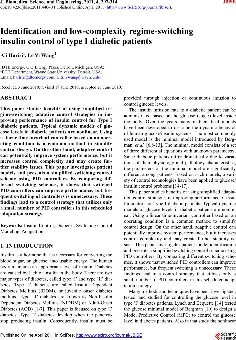J. Biomedical Science and Engineering, 2011, 4, 297-314 JBiSE
doi:10.4236/jbise.2011.44040 Published Online April 2011 (http://www.SciRP.org/journal/jbise/).
Published Online April 2011 in SciRes. http://www.scirp.org/journal/JBiSE
Identification and low-complexity regime-switching
insulin control of type I diabetic patients
Ali Hariri1, Le Yi Wang2
1DTE Energy, One Energy Plaza, Detroit, Michigan, USA;
2ECE Department, Wayne State University, Detroit, USA.
Received 3 June 2010; revised 19 June 2010; accepted 21 June 2010.
ABSTRACT
This paper studies benefits of using simplified re-
gime-switching adaptive control strategies in im-
proving performance of insulin control for Type I
diabetic patients. Typical dynamic models of glu-
cose levels in diabetic patients are nonlinear. Using
a linear time invariant controller based on an oper-
ating condition is a common method to simplify
control design. On the other hand, adaptive control
can potentially improve system performance, but it
increases control complexity and may create fur-
ther stability issues. This paper investigates patient
models and presents a simplified switching control
scheme using PID controllers. By comparing dif-
ferent switching schemes, it shows that switched
PID controllers can improve performance, but fre-
quent switching of controllers is unnecessary. These
findings lead to a control strategy that utilizes only
a small number of PID controllers in this scheduled
adaptation strategy.
Keywords: Insulin Control; Diabetes; Switching Control;
Modeling; Adaptation
1. INTRODUCTION
Insulin is a hormone that is necessary for converting the
blood sugar, or glucose, into usable energy. The human
body maintains an appropriate level of insulin. Diabetes
are caused by lack of insulin in the body. There are two
major types of diabetes, called type ‘I’ and type ‘II’ dia-
betes. Type ‘I’ diabetes are called Insulin Dependent
Diabetes Mellitus (IDDM), or juvenile onset diabetes
mellitus. Type ‘II’ diabetes are known as Non-Insulin
Dependent Diabetes Mellitus (NIDDM) or Adult-Onset
Diabetes (AOD) [1-7]. This paper is focused on type ‘I’
diabetes. Type ‘I’ diabetes develop when the pancreas
stop producing insulin. Consequently, insulin must be
provided through injection or continuous infusion to
control glucose levels.
The insulin infusion rate to a diabetic patient can be
administrated based on the glucose (sugar) level inside
the body. Over the years many mathematical models
have been developed to describe the dynamic behavior
of human glucose/insulin systems. The most commonly
used model is the minimal model introduced by Berg-
man, et al. [6,8-13]. The minimal model consists of a set
of three differential equations with unknown parameters.
Since diabetic patients differ dramatically due to varia-
tions of their physiology and pathology characteristics,
the parameters of the minimal model are significantly
different among patients. Based on such models, a vari-
ety of control technologies have been applied to glucose/
insulin control problems [14-17].
This paper studies benefits of using simplified adapta-
tion control strategies in improving performance of insu-
lin control for Type I diabetic patients. Typical dynamic
models of glucose levels in diabetic patients are nonlin-
ear. Using a linear time-invariant controller based on an
operating condition is a common method to simplify
control design. On the other hand, adaptive control can
potentially improve system performance, but it increases
control complexity and may create further stability is-
sues. This paper investigates patient model identification
and presents a simplified switching control scheme using
PID controllers. By comparing different switching sche-
mes, it shows that switched PID controllers can improve
performance, but frequent switching is unnecessary. These
findings lead to a control strategy that utilizes only a
small number of PID controllers in this scheduled adap-
tation strategy.
Many methods and techniques have been investigated,
tested, and studied for controlling the glucose level in
type ‘I’ diabetes patients. Lynch and Bequette [14] tested
the glucose minimal model of Bergman [10] to design a
Model Predictive Control (MPC) to control the glucose
level in diabetes patients. Also in that study the nonlinear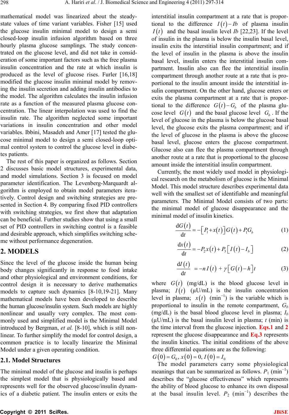

A. Hariri et al. / J. Biomedical Science and Engineering 4 (2011) 297-314 298
mathematical model was linearized about the steady-
state values of time variant variables. Fisher [15] used
the glucose insulin minimal model to design a semi
closed-loop insulin infusion algorithm based on three
hourly plasma glucose samplings. The study concen-
trated on the glucose level, and did not take in consid-
eration of some important factors such as the free plasma
insulin concentration and the rate at which insulin is
produced as the level of glucose rises. Furler [16,18]
modified the glucose insulin minimal model by remov-
ing the insulin secretion and adding insulin antibodies to
the model. The algorithm calculates the insulin infusion
rate as a function of the measured plasma glucose con-
centration. The linear interpolation was used to find the
insulin rate. The algorithm neglected some important
variations in insulin concentration and other model
variables. Ibbini, Masadeh and Amer [17] tested the glu-
cose minimal model to design a semi closed-loop opti-
mal control system to control the glucose level in diabe-
tes patients.
The rest of this paper is organized as follows. Section
2 discusses basic model structures, experimental data,
and model simulations. Section 3 is focused on model
parameter identification. The Levenberg-Marquardt al-
gorithm is employed to obtain model parameters itera-
tively. Control design and switching strategies are pre-
sented in Section 4. By comparing fixed PID controllers
with switching strategies, we first show that adaptation
can be beneficial. Further studies show that using a small
set of PID controllers in switching control is a feasible
and desirable approach, which simplifies switching sche-
me without performance degeneration.
2. MODELS
Since the level of the glucose inside the human being
body changes significantly in response to food intake
and other physiological and environment conditions, for
control design it is necessary to derive mathematics
models to capture such dynamics [8-10,19-21]. Many
mathematical models have been developed to describe
the human glucose/insulin system. Such models are highly
nonlinear and usually very complex. The most com-
monly used and simplified model is the Minimal Model
introduced by Bergman, et al. [8-10], which is still non-
linear. To further simplify the model for control design, a
common practice is to locally linearize the Minimal
Model under a given operating condition.
2.1. Model Structures
The minimal model of the glucose and insulin is perhaps
the simplest model that is physiologically based and
represents well for the observed glucose/insulin dynam-
ics of a diabetic patient. The insulin enters or exits the
interstitial insulin compartment at a rate that is propor-
tional to the difference

I
tIb of plasma insulin


I
t and the basal insulin level Ib [22,23]. If the level
of insulin in the plasma is below the insulin basal level,
insulin exits the interstitial insulin compartment; and if
the level of insulin in the plasma is above the insulin
basal level, insulin enters the interstitial insulin com-
partment. Insulin also can flee the interstitial insulin
compartment through another route at a rate that is pro-
portional to the insulin amount inside the interstitial in-
sulin compartment. On the other hand, glucose enters or
exits the plasma compartment at a rate that is propor-
tional to the difference

b
Gt G of the plasma glu-
cose level


Gt and the basal glucose level b G. If the
level of glucose in the plasma is below the glucose basal
level, the glucose exits the plasma compartment; and if
the level of glucose in the plasma is above the glucose
basal level, glucose enters the glucose compartment.
Glucose also can flee the plasma compartment through
another route at a rate that is proportional to the glucose
amount inside the interstitial insulin compartment.
Currently, the most widely used model in physiologi-
cal research on the metabolism of glucose is the Minimal
Model. This model structure describes experimental data
well with the smallest set of identifiable and meaningful
parameters. The Minimal Model consists of two parts:
the minimal model of glucose disappearance and the
minimal model of insulin kinetics.

 
11
d
db
Gt Pxt GtPG
t 
 (1)

 
23
d
db
xt Px tPItI
t 

(2)

 
d +
d
It nItG tht
t
   

(3)
where


Gt (mg/dL) is the blood glucose level in
plasma;


I
t (µU/mL) is the insulin concentration
level in plasma;


x
t (min−1) is the variable which is
proportional to insulin in the remote compartment, Gb
(mg/dL) is the basal blood glucose level in plasma; Ib
(µU/mL) is the basal insulin level in plasma; t (min) is
the time interval from the glucose injection. Eqs.1 and 2
represent the glucose disappearance and Eq.3 represents
the insulin kinetics. The initial conditions of the above
three differential equations are as the following:






00
0,00,0GGxI I


The model parameters carry some physiological
meanings that can be summarized as follows. P1 (min−1)
describes the “glucose effectiveness” which represents
the ability of blood glucose to enhance its own disposal
at the basal insulin level. P2 (min−1) describes the

A. Hariri et al. / J. Biomedical Science and Engineering 4 (2011) 297-314 299
decreasing level of insulin action with time. P3 (2 min



1
UmL ) describes the rate in which insulin action is
increased as the level on insulin deviates from the corre-
sponding baseline.  ((µU/mL)(mg/dL)−1min−1) de-
notes the rate at which insulin is produced as the level of
glucose rises above a “target glycemia” level. n (min−1)
represents fractional insulin clearance. h (mg/dL) is the
pancreatic “target glycemia” level. G0 (mg/dL) is the
theoretical glucose concentration in plasma extrapolated
to the time of glucose injection t = 0 [8-10,24]. I0
(µU/mL) is the theoretical plasma insulin concentration
at t = 0. µU/mL is the conventional unit to measure the
insulin level and has the following conversion formula: 1
micro-unit/ milliliter = 6 picomole/liter (1µU/mL = 6
pmol/L) [25,26]. P1, P2, P3, n,  , h, G0 and I0 are the pa-
rameters to be estimated.
A fourth differential equation will be added to the set
of the Minimal Model equations to represent a first-order
pump dynamics:
  

1
1
d1
d
Ut Ut ut
ta
 (4)
where

1
Ut is the infusion rate,

ut is the input
command, and a is the time constant of the pump.
2.2. Experimental Data
A new approach was developed by Bergman, et al. [8-10]
to compute the pancreatic responsiveness and insulin
sensitivity in the intact organism. This approach uses
computer modeling to investigate the plasma glucose
and insulin dynamics during a Frequently Sampled In-
travenous Glucose Tolerance (FSIGT). An amount of
glucose was injected at t = 0 over a period of time equal
to 60 seconds [8-10,27]. The blood samples were taken
from a fasting subject at regular intervals of time, and
then analyzed for glucose and insulin content. Glucose
was measured in triplicate by the glucose oxidize tech-
nique on an automated analyzer. The coefficient of vari-
ation of a single glucose determination was about ±
1.5%. Insulin was measured in duplicate by radioimmu-
noassay, with dextrin-charcoal separation using a human
insulin standard. Table 1 shows the FSIGT test data for a
normal individual.
2.3. Model Simulation
Implementation of the minimal model can be achieved
by using computer simulation tools. The two differential
Eqs.1 and 2 of the minimal model that correspond to the
glucose kinetics are modeled here by using the MAT-
LAB/Simulink software. In this model, the insulin


I
t
is considered as an input and the glucose


Gt as an
output. The values of the input

I
t at a time interval
are given in Table 1. The simulation diagram of the
minimal model for the glucose kinetic is shown in Fig-
ure 1. The output of the system, glucose


Gt , is
Table 1. FSIGT test data for a normal individual.
Sampling time
(minutes)
Glucose level
(mg/dL)
Insulin level
(µU/mL)
0
2
4
6
8
10
12
14
16
19
22
27
32
42
52
62
72
82
92
102
122
142
162
182
92
350
287
251
240
216
211
205
196
192
172
163
142
124
105
92
84
77
82
81
82
82
85
90
11
26
130
85
51
49
45
41
35
30
30
27
30
22
15
15
11
10
8
11
7
8
8
7
shown in Figure 2 for a normal individual with the fol-
lowing parameters: P1 = 3.082 × 10–2, P2= 2.093 × 10–2,
P3 = 1.062 × 10–5, G0 = 350, Gb = 92, Ib = 11, [8-10].
3. PARAMTERS ESTIMATION
3.1. Parameter Estimation
Parameter estimation is to determine the values of model
parameters that provide the best fit to measured data, based
on some error criteria such as least-squares. The method of
least squares assumes that the best-fit curve of a given set of
data is the curve that has the minimal sum of the deviations
squared from a given set of data [28-31]. Given a set of data
(x1, y1), (x2, y2), (x3, y3),

, (xN, yN), where the independent
variable is x and the dependent variable is y, under a se-
lected model function form

f
x the least squares (LS)
estimation seeks to minimize

2
1
N
ii
i
yfx


  


 (5)
When the function is an m-th degree polynomial


2
01 2
m
m
fxaax axax  (6)
we have


2
1
2
2
01 2
1
N
ii
i
Nm
iiimi
i
yfx
yaaxax ax


  








(7)
The unknown coefficients 012
,, , ,
m
aaa a , can be
estimated to yield a least squares error.

A. Hariri et al. / J. Biomedical Science and Engineering 4 (2011) 297-314 300
Figure 1. Simulation diagram of the glucose kinetic model.
Figure 2. The output of the minimal model for the glucose
kinetics
Model parameters can be obtained iteratively to re-
duce computational complexity. It starts with an initial
guess of the unknown parameters. Each iteration updates
the current estimate based on new observations. Suppose
there are m base functions12
, ,,m ff f of n parameters
12
, ,,n pp p . The functions and the parameters can be
represented as follows:


T
12
T
12
, ,,
, ,,
m
n
f
ff
pp p
 
 
f
p (8)
The least square method is to find the values of the
unknown parameters 12 , ,,n pp p for which the cost
function is minimum, i.e.
 
T2
1
11
22
m
i
i
Sf



Pff p (9)
The Levenberg-Marquardt algorithm is an iterative
technique that seeks the minimum of a multivariate
function that is expressed as the sum of squares of
nonlinear real-valued functions [28]. It has become a
standard technique for nonlinear least-squares problems.
Levenberg-Marquardt can be thought of as a combina-
tion of steepest descent and the Gauss-Newton method.
When the current solution is far from the correct one, the
algorithm behaves like a steepest descent method which
is guaranteed to converge. When the current solution is
close to the correct solution, it becomes a Gauss-Newton
method.
The Levenberg-Marquardt algorithm is an iterative
procedure. Let


ˆfxp be the parametrized model
function. The minimization starts after an initial guess
for the parameter vector p is provided. The algorithm is
locally convergent, namely it converges when the initial
guess is close to the true values. In each iteration step,
the parameter vector p is updated by a new esti-
mate


p, where

is a small correction term that can
be determined by a Taylor Series expansion which leads
to the following approximation:



p
p
ff 

 ppJ (10)

A. Hariri et al. / J. Biomedical Science and Engineering 4 (2011) 297-314 301
where,
J
is the Jacobian of f at p

f

p
Jp (11)
Levenberg-Marquardt iterative initiates at the starting
point 0 p, and produces a series of vectors 123 , ,pp p
etc, that converge towards a local minimizer p

of f.
At each step, it is required to find the

which mini-
mizes the value of


p
p
ff 

 xp xpJ
That gives the following:

ˆ
p
pp
fe 

 xp xxJJ (12)
where
p

is the solution to a linear least squares prob-
lem. The minimum is achieved when the term pe


J
is orthogonal to column space J. Based on that, the fol-
lowing can be concluded

T0
pe
 JJ (13)
Eq.13 can be rearranged as the following

TT
pee

J
JJ (14)
The Levenberg-Marquardt algorithm solves a slight
variation of Eq.14, which is known as the augmented
normal equation
T
pe
 NJ (15)
where the diagonal elements of N are computed
as T
ii ii



 NJJfor 0

, while the rests of the
matrix N are identical to those of the matrix T


J
J.

is called the damping parameter. If the updated parame-
ter vector,
p


p, where
p

is computed from Eq.15,
yields a reduction in the residual value or error e, then
the update is valid and the process repeats with a de-
creased damping parameter

. Otherwise, the damping
parameter is increased and the augmented normal Eq.15
is solved again. Then the process iterates until a value of
p

that reduces error is found. The MATLAB Software
has the Optimization Toolbox which has a command
called Lsqnonlin for this algorithm.
This algorithm is applied to our problem here. The
FSIGT data sample in Table 1 consists of 24 samples.
The FSIGT samples were taken over a period of 182
minutes. The unknown parameters of the minimal model
Eq.1, Eq.2, Eq.3 were estimated by utilizing the Le-
venberg-Marquadrt Algorithm. The parameters to be es-
timated were given an initial guess, then the algorithm
was used to update the parameters using the sequential
data in Table 1. A MATLAB program was written to
estimate the unknown parameters. The estimated values
of those parameters are shown in Table 2.
Table 2. Estimated Parametres.
Parameters Normal
Individual #1
Normal
Individual #2
P1
P2
P3
n
γ
h
G0
I0
0.032299
0.0092644
5.3004e–006
0.29858
0.0068676
90.3709
295.6801
401.7177
0.049519
41.5953
1.8577e–004
0.14653
1.0113e–005
196.0531
318.84
203.2434
The values of the parameters shown in Ta b l e 2 were
implemented in the simulation diagram of the minimal
model shown on Figure 1. The values of the glucose
levels of both individuals are shown in Table 3.
The graphs of both experimental and simulated data
for normal individual #1 and #2 are shown in Figure 3
and Figure 4 respectively.
These plots show that the two graphs (experimental
and simulated) are close to each other, leading to the
conclusion that the estimated values of parameters are
close to the actual values. In general, the relative errors
indicate how good an estimate is, relative to the true
values. Although absolute errors are useful, they do no
necessarily give an indication of the importance of an
error. If the experimental value is denoted by G, and
the estimated (or simulated) value is denoted by G,
then the relative error is defined as
Relative Error
ˆ
GG
G

 (16)
Table 3. Simulated data for normal individuals #1 and #2.
Normal Individual
#1
Normal Individual
#2
Sampling time
during the test
(minutes) Glucose Level
(mg/dL)
Glucose Level
(mg/dL)
0
2
4
6
8
10
12
14
16
19
22
27
32
42
52
62
72
82
92
102
122
142
162
182
94
295.6801
282.1308
268.2993
254.8580
242.1020
230.1353
218.9702
208.5776
198.9116
185.6659
173.7810
156.6159
142.2917
120.5167
105.8327
96.35277
90.67314
87.73594
86.65621
86.77255
89.03143
92.55181
95.65837
94
318.84
297.2223
277.7749
260.2561
244.4545
230.1878
217.2973
205.6436
195.1034
181.1443
169.1246
152.6775
139.8434
122.0036
111.1272
104.4947
100.4500
97.98329
96.47894
95.56149
94.66075
94.32573
94.20113

A. Hariri et al. / J. Biomedical Science and Engineering 4 (2011) 297-314 302
020 4060 80100 120 140160 18020
0
0
50
100
150
200
250
300
350
400
time (min)
Glucose mg/ dL)
p
Basal Level
E x perim ental Data
Simulated Data
Figure 3. Plot of glucose level G(t) for normal individual #1.

020 40 6080100120 140160180 20
0
0
50
100
150
200
250
300
350
400
time (min)
Glucose mg/ dL)
p
B asal Level
E xperim ental Data
Simulated Data
Figure 4. Plot of glucose level G(t) for normal individual #2.
And the Square Relative Error can be expressed as
Square Relative Error
2
ˆ
GG
G





(17)
When the data is sampled over a certain period of time,
the mean squared relative error (MSRE) can be used.
The MSRE is defined as
2
1
ˆ
1
MSRE, for 1, 2,,
n
ii
ii
GG in
nG







 (18)
where i G is the experimental value at sample i. ˆ
i
G is
the estimated value at sample i. n is the number of sam-
ples of a data set.
The Square Relative Error between the experimental
data and the simulated data of the glucose level for indi-
vidual #1 and # 2 are calculated and shown in Ta ble 4
and Table 5 respectively. Normally the Mean Square
Relative Error is expressed in percentage format. Below
is the percentage error for both individuals: the percent-
Table 4. Error data for normal individuals #1.
Experimental
Data, G(t)
Simulated
Data, ˆ()Gt
Square Relative
Error
94
298
284
272
253
248
235
217
208
205
191
172
164
141
132
120
116
108
106
104
105
109
107
110
94
295.6801
282.1308
268.2993
254.8580
242.1020
230.1353
218.9702
208.5776
198.9116
185.6659
173.7810
156.6159
142.2917
120.5167
105.8327
96.35277
90.67314
87.73594
86.65621
86.77255
89.03143
92.55181
95.65837
0
6.060466e–005
4.3317e–005
0.0001851148
5.393524e–005
0.0005656016
0.0004285321
8.243416e–005
7.710311e–006
0.0008820624
0.0007799362
0.0001072176
0.002027272
8.391868e–005
0.007568141
0.01393832
0.0286871
0.02573902
0.02968814
0.02781129
0.03013514
0.03356148
0.01823304
0.01699855
Table 5. Error data for normal individuals #2.
Experimental
Data, G(t)
Simulated
Data, ˆ() Gt
Square Relative
Error
94
320
303
289
272
258
244
223
205
194
182
169
152
139
122
112
105
100
98
97
97
95
94
93
94
318.84
297.2223
277.7749
260.2561
244.4545
230.1878
217.2973
205.6436
195.1034
181.1443
169.1246
152.6775
139.8434
122.0036
111.1272
104.4947
100.4500
97.98329
96.47894
95.56149
94.66075
94.32573
94.20113
0
1.314063e–005
0.0003635986
0.001508629
0.001864179
0.002756472
0.003204405
0.0006539557
9.857924e–006
3.235126e–005
2.210359e–005
5.439401e–007
1.986409e–005
3.681781e–005
8.715616e–010
6.073247e–005
2.315634e–005
2.024906e–005
2.909034e–008
2.88559e–005
0.0002199282
1.275242e–005
1.200794e–005
0.0001668063
age MSRE for individual # 1 = 0.99028%; the percent-
age MSRE for individual # 2 = 0.04596%.
3.2. Model Linearization
Now let us recall the four differential Eqs.1-4 that define
the proposed mathematical model and denote them as


1
f
G,


2
f
x,


3
f
I, and

41
f
U. The result is

A. Hariri et al. / J. Biomedical Science and Engineering 4 (2011) 297-314 303
  
111
d
db
Gt
f
GPxtGtPG
t
 
 (19)
   
223
d
db
xt
f
xPxtPItI
t
 



 (20)
   
31
d
d
It
f
InItGthtUt
t
  
 (21)
   
1
41 1
d1
d
Ut
f
UUtUt
ta
 (22)
The above equations can be written and arranged as
follows.
The above equations can be further simplified as
 
11 1b
f
GPGtxtGt PG (23)




2233b
f
xPxtPItPI (24)
  
31
f
InIttGthtUt    (25)
  
41 1
11
f
UUtUt
aa
 (26)
The above system is a nonlinear system due to the
presence of the nonlinear term that appears in Eq.23.
The nonlinear term is



x
tGt. Now let us make the
following definitions
  


12341
,,,
x
t Gtxt xtxtItxt ut
Then Eqs.23 to 26 become


1
111 21
d
db
xt
P
xt xtxt PG
t (27)

 
2
2233 3
d
db
xt Px tPxtPI
t (28)

 
3
134
d
d
xt tx tnxtxtht
t


(29)

 
4
4
d11
d
xt
x
tut
taa
 (30)
The Jacobian matrices (
x
J
and u
J
) of the model
can be derived as
12 1
23
00
0 0
0 0
0 1
1
0 0 0
,
x
Px x
PP
tn
a
x
xuu
 













J
and
00
0
0
0
1
,
u
a
x
xuu









J (31)
where the point (x0, u
0) is the equilibrium point. The
equilibrium point can be calculated by setting the state
equations to zero and solving
11010 2010 b
PxxxPG

 (32)
220 330 30 b
PxPx PI

 (33)
1030 400tx nxxht


  (34)
40 0
11
0xu
aa

 (35)
where x10, x20, x30, x40 and u0 are the values of the state
variables and the input at the operating point (i.e. the
equilibrium point). At the equilibrium point, u0 = 0,
Eq.35 becomes 40
10x
a

, that gives
x40 = 0 (36)
Substituting the value of x40 in Eq.34 results in
10 300tx nxht


 and


10
30
x
ht
xn


 (37)
The value of x30 can be substituted in Eq.33


10
220 330 b
xht
Px PPI
n
 


to obtain
31033
20
222
b
PtxPth PI
xPnPn P

 (38)
Now, by substituting the value of 20
x
in Eq.32 we have

2
333
10110 1
222
0
b
b
PtPthPI
xP xPG
PnPn P



 


(39)
The above equation is a 2nd order equation and can be
solved by using the quadratic formula
2
10
4
2
bb ac
xa
 

(40)
where 333
11
222
,,
b
b
PtPth PI
abP cPG
PnPn P

 
There are 2 possible values of x10. Since x20 and x30 are
expressed in term of x10, there will be 2 possible values
for each. Based on that, the controllability test will be
studied to check which value of x10 is accepted.
3.3. A Case Study
The simulation diagram shown in Figure 1 was used to
simulate the data of a diabetic patient. The value of the
parameters for a diabetic patient is shown below. P1 = 0,
P2 = 0.81/100, P3 = 4.01/1000000, I0 = 192, G0 = 337, 
= 2.4/1000, h = 93, n = 0.23, a = 2, Gb = 99, Ib = 8, [10].

A. Hariri et al. / J. Biomedical Science and Engineering 4 (2011) 297-314 304
The output of the simulated system is shown in Figure 5.
By examining Figure 5, it can be clearly seen that the
glucose level does not come down to the basal level after
injecting an amount of 337 mg/dL of glucose inside a
diabetic patient. Figure 5 shows that the level of the
glucose inside a diabetic patient decreases for the first
100 minutes, starts increasing afterward, and reaches the
value of around 310 mg/dL after 3 hours from the time
the glucose was injected. The goal is to bring down the
value of the glucose inside a diabetic patient to the nor-
mal level or at least into a small neighborhood of the
basal level. The above goal can be achieved by design-
ing a PID feedback controller. The controller is to regu-
late the infusion rate and inject the required amount of
the insulin inside the diabetic patient, and in turn the
insulin will work inside the patient to bring down the
level of glucose to the normal level or at least to the
neighborhood of the normal level.
4. CONTOL DESIGN
We start with a linearized state space model for our sys-
tems. The general form of the state space is defined in
the following equation:
x
xu
yxu


AB
CD

(41)
The proposed mathematical model at the equilibrium
point (x0, u
0) can be written in the state space form as
shown below:
120 10
23
0 00
0 00
0
0 1
1 1
0 0 0
Px x
PP
xx
tn
a a




 

















1 0 0 0
u
yx



(42)
Figure 5. Output of the simulated system for diabetic.
where u is the input and y is the output of the system.
The data of a diabetic person shown in Section 3.3 was
used and the equilibrium point (x0, u0) was calculated as
time varies from t = 1 min to t = 182 min. The two val-
ues for x10 that were calculated before were substituted
in Eq.42 and the controllability test was performed. It
was found that only one value (the one obtained from the
sign) makes the system to be controllable, hence only
this value is used in the subsequent development.
4.1. Design of PID Controllers for Diabetic
Patient
When designing a controller, the designer must define
the specifications that need to be achieved by the con-
troller. Normally the maximum overshoot (Mp) of the
system step response should be small. Commonly a
range between 10% and 20% is acceptable. Also the set-
tling time (ts), is an important factor. The objective here
is to design a PID controller, so that the closed-loop sys-
tem has the following specifications: small steady-state
error for a step input; less than 10% overshoot; settling
time less than 60 minutes.
The patient dynamic system was expressed in the state
space representation in (42). For an overshoot less than
10%, a damping ratio must be greater than 0.59, and a
settling time less than 60 minutes implies that


n


must be greater than 0.067.
The PID Controllers can be designed based on the
models at different operating points. The following list
contains the models at t = 1, 20, 40, 60, 90, 120, 150 and
182 minutes, and the corresponding PID controllers.
Since B and C do not change with time, they are fixed in
all cases as:

0
0
and 1 0 0 0
0
0.5







BC
The control design is done by applying the root locus
method and then evaluated by using the step response.
For example, if the model at t = 1 min is used, after sub-
stituting the above numerical values (42), the root locus
plot can be generated by the Matlab functions
MATLAB Program
Plotting the open loop system Root locus
using MATLAB
[num, den] = ss2tf(A,B,C,D];
rlocus(num, den)
axis([–0.6 0.1 –0.5 0.5])
sgrid(0.59,0)
sigrid(0.067)

A. Hariri et al. / J. Biomedical Science and Engineering 4 (2011) 297-314 305
The open loop poles are shown in Figure 6. These
poles are located at –0.0040 + 0.0045j, –0.0040 –
0.0045j, –0.2302, –0.5. The four poles are stable, but the
first two poles are very close to the imaginary axis and
hence represent the slowest dynamics. The controller
takes the form
 
12
K
Sz Sz
Gc SS


where K is the value of the gain where the root locus
intersects with the line of the damping ratio. The z1 and
z2 represent the value of the zeros to be added and may
be selected to cancel the slowest poles of the dynamic
system. Hence, select z1 = –0.004 + 0.0045j, z2 = –0.004
– 0.0045j.
The controller is * (please see the equation below)
resulting in the system matrix A and the PID controller
as
1
0 859.6667 0 0
0 0.0081 0.00000401 0
0.0024 0 0.23 1
0 0


 A


2
1
,
0 0.5
0.008 0.00003625
C
KS S
GS S









The PID Parameters are:
4
0.0444, 2.009410, 5.59
pi d
KK K


The design specifications of the system require the
maximum overshoot to be less than 10% and the settling
time to be less than 60 minutes. After inserting the PID
controller in series with the patient system and connect-
ing them in a unity feedback, we get the maximum
overshoot 5.71% and the settling time 47.5 minutes (see
Figure 7).
t = 20 minutes:
20
0 131.33 0 0
0 0.0081 0.00000401 0
0.048 0 0.23 1
0


 A


2
20
,
0 0 0.5
0.0076 0.0001
C
KS S
GS S









The PID Parameters are:
= 0.2160, 0.0031, = 28.4
pi d
KKK
Figure 6. Output of the simulated system for Root Locus.
Figure 7. Output of the unit step response, using the model at
t= 1 minute with K = 5.5.
t = 40 minutes:
40
0 112.17 0 0
0 0.0081 0.00000401 0
0.096 0 0.23 1
0


 A


2
40
,
0 0 0.5
0.0072 0.0002
C
KS S
GS S















The PID Parameters are:
= 0.2374, 0.0061, = 32.7
pid
KKK

*
 





0.0040 0.00450.0040 0.0045
K
SjSj
Gc SS
 


A. Hariri et al. / J. Biomedical Science and Engineering 4 (2011) 297-314 306
t = 60 minutes:
60
0 105.78 0 0
0 0.0081 0.00000401 0
0.1440 0 0.23 1
0


 A


2
60
,
0 0 0.5
0.0070.0003
C
KS S
GS S









The PID Parameters are:
4
0.0444, 2.009410, 5.59
pi d
KKK


t = 90 minutes:
90
0 101.52 0 0
0 0.0081 0.00000401 0
0.2160 0 0.23 1
0


 A


2
90
,
0 0 0.5
0.0064 0.0004
C
KS S
GS S









The PID Parameters are:
= 0.2331, 0.0138, = 36.4
pi d
KK K
t = 120 minutes:
120
0 99.39 0 0
0 0.0081 0.00000401 0
0.288 0 0.23 1
0 0


 A


2
120
,
0 0.5
0.0058 0.0005
C
KS S
GS S









The PID Parameters are:
= 0.2234, 0.0187, = 37.9
pi d
KKK
t = 150 minute:
150
0 98.11 0 0
0 0.0081 0.00000401 0
0.36 0 0.23 1
0 0


 A


2
150
,
0 0.5
0.0054 0.0006
C
KS S
GS S









The PID Parameters are:
= 0.2032, 0.0229, = 37.7
pi d
KKK
t = 182 minute:
182
0 97.21 0 0
0 0.0081 0.00000401 0
0.4368 0 0.23 1
0 0


 A


2
182
,
0 0.5
0.0048 0.0007
C
KSS
GS S















The PID Parameters are:
= 0.1870, 0.0281, = 38.5
pid
KK K

4.2. Individual PID Controllers
Non-adaptive PID controllers use a fixed PID controller
for the entire control period and rely on its robustness to
maintain control performance. For each individual PID
controller (with its transfer function found in the previ-
ous subsection for t = 1, 20, 40, 60, 90, 120, 150 and
182 min) the simulation results on

Gt and


ut are
shown below in Figur es 8-15.
Under the individual PID controllers, the output


Gt, the glucose level, did not really meet the design
specification, and the glucose level is not near or at least
in a small neighborhood of the glucose basal level. The
overshoot of the system was too high and beyond the
acceptable level. Also the settling time was not even
close to where it should be as per the design requirement.
And the steady state error was not satisfactory. A new
method should be developed and implemented to meet
all the design specifications. This method is explained in
detail in the following section.
4.3. Switched PID Controllers
The individual PID controllers could not lower the glu-
cose level


Gt of the patient to the neighborhood of
the glucose basal level. Consequently, we introduce a
new control-switching scheme that adapts controllers to
meet design specifications. The switching control con-
sists of the following items: One “time clock,” one
“switch case” block, one “if action case” block, one
“merge” block, and eight “off-on switches.” All these
blocks are connected together to form the wiring dia-
gram of the Control-Switching Scheme.
The functions of the control switching scheme is de-
tailed in Figure 16. The “Time Clock” is to provide the
“Switch Case” block with time as a signal input to acti-
vate it.
The “Switch Case” block receives a single input from
the clock, which it uses to form case conditions that de-
termine which subsystem to execute. Each output port
case condition is attached to a Switch Case Action sub-

A. Hariri et al. / J. Biomedical Science and Engineering 4 (2011) 297-314 307
Figure 8.

Gt and

ut using 1
C
G.
Figure 9.

Gt and

ut using 20
C
G.
Figure 10.

Gt and

ut using 40
C
G.

A. Hariri et al. / J. Biomedical Science and Engineering 4 (2011) 297-314 308
Figure 11.


Gt and

ut using 60
C
G.
Figure 12.


Gt and

ut using 90
C
G.
Figure 13.


Gt and

ut using 120
C
G.

A. Hariri et al. / J. Biomedical Science and Engineering 4 (2011) 297-314 309
Figure 14.


Gt and


ut using 150
C
G.
Figure 15.

Gt and

ut using 182
C
G.
Figure 16. Control-Switching Scheme Simulation Diagram.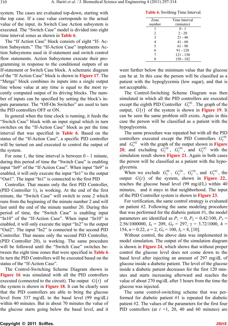

A. Hariri et al. / J. Biomedical Science and Engineering 4 (2011) 297-314 310
system. The cases are evaluated top-down, starting with
the top case. If a case value corresponds to the actual
value of the input, its Switch Case Action subsystem is
executed. The “Switch Case” model is divided into eight
time interval zones as shown in Table 6.
The “If Action Case” block consists of eight “If- Ac-
tion Subsystem.” The “If-Action Case” implements Ac-
tion Subsystems used in if-statement and switch control
flow statements. Action Subsystems execute their pro-
gramming in response to the conditional outputs of an
If-statement or Switch Case block. A schematic diagram
of the “If Action Case” block is shown in Figure 17. The
“Merge” block combines its inputs into a single output
line whose value at any time is equal to the most re-
cently computed output of its driving blocks. The num-
ber of inputs can be specified by setting the block’s in-
puts parameter. The “Off-On Switches” are used to turn
the PID controllers OFF or ON.
In general when the time clock is running, it feeds the
“Switch Case” block with an input signal which in turn
switches on the “If-Action Case” block as per the time
interval that was specified in Table 6. Based on the
status of the “If-Action Case”, a specific PID controller
will be turned on and executed to control the output of
the system.
For zone 1, the time interval is between 0 - 1 minute,
during this period of time the “Switch Case” is enabling
input “In9” of the “If-Action Case”. When input “In9” is
enabled, it will only execute the input “In1” to the output
“Out1”. The input “In1” is connected to the first PID
Controller. That means only the first PID Controller,
(PID Controller 1), is working. At the end of the first
minute, the “Switch Case” will switch to zone 2 which
runs from the beginning of the minute number 2 and will
last until the end of the minute number 20. During this
period of time, the “Switch Case” is enabling input
“In10” of the “If-Action Case”. When input “In10” is
enabled, it will only execute the input “In2” to the output
“Out2”. The input “In2” is connected to the second PID
Controller. That means only the second PID Controller,
(PID Controller 20), is working. The same procedure
will be followed until the “Switch Case” switches be-
tween the eight time zones that were specified in Table 6.
In turn the PID Controllers will be executed based on the
status of the “If-Action Case”.
The Control-Switching Scheme Diagram shown in
Figure 16 was simulated with all the PID controllers
executed (connected to the circuit). The output


Gt of
the system is shown in Figure 18. It can be clearly seen
that the PID controllers are able to bring the glucose
level from 337 mg/dL to the basal level (99 mg/dL)
within 40 minutes. But in about 70 minutes the value of
the glucose starts going below the basal level, and it
Table 6. Swithing Time Interval.
Zone
number
Time Interval
(minutes)
1 0 - 1
2 2 - 20
3 21 - 40
4 41 - 60
5 61 - 90
6 91 - 120
7 121 - 150
8 150 - 182
went further below the minimum value that the glucose
can be at. In this case the person will be classified as a
patient with the hypoglycemia (low sugar), and that is
not acceptable.
The Control-Switching Scheme Diagram was then
simulated in which all the PID controllers are executed
except the eighth PID Controller 182
C
G. The graph of the
output,


Gt of the system is shown in Figure 19. It
can be seen the same problem still exists. Again in this
case the person will be classified as a patient with the
hypoglycemia.
The same procedure was repeated but with all the PID
controllers executed except the PID Controllers 150
C
G
and 182
C
G with the graph of the output shown in Figure
20; and excluding 120
C
G, 150
C
G, and 182
C
G with the
simulation result shown Figure 21. Again in both cases
the person will be classified as a patient with the hypo-
glycemia.
When we exclude 90
C
G, 120
C
G, 150
C
G, and 182
C
G, the
output


Gt of the system, shown in Figure 22,.
reaches the glucose basal level (99 mg/d/L) within 40
minutes, and it stays in that neighborhood. The input
of the PID Controller system is shown in Figure 23.
For verification, the same control strategy is evaluated
on patient #2. Following the same modeling procedure
that was performed for the diabetic patient #1, the model
parameters are identified as P1 = 0, P2 = 0.42/100, P3 =
2.56/1000000, I0 = 209, G0 = 297,  = 3.72/1000, h =
154, n = 0.22, a = 2, Gb = 100, Ib = 8, [10].
Without control, the above data was implemented in
model simulation. The output of the simulation diagram
is shown in Figure 24, which shows that without proper
control the glucose level does not come down to the
basal level after injecting an amount of 297 mg/dL of
glucose inside a diabetic patient. The level of the glucose
inside a diabetic patient decreases for the first 120 min-
utes and starts increasing afterward and reaches the
value of about 270 mg/dL after 3 hours from the time the
glucose was injected.
The same control-switching scheme that was per-
formed for diabetic patient #1 is repeated for diabetic
patient #2. The values of the parameters for the first four
PID controllers (at t =1, 20, 40 and 60 minutes) are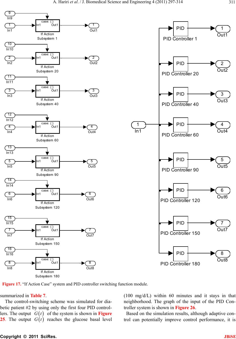

A. Hariri et al. / J. Biomedical Science and Engineering 4 (2011) 297-314 311

8
Out8
7
Out7
6
Out6
5
Out5
4
Out4
3
Out3
2
Out2
1
Out1
PID
PI D Controller 90
PID
PI D Controller 60
PID
PI D Controller 40
PID
PI D Controller 20
PID
PID Controller 180
PID
PID Controller 150
PID
PID Controller 120
PID
PI D Controller 1
1
In1
8
Out8
7
Out7
6
Out6
5
Out5
4
Out4
3
Out3
2
Out2
1
Out1
case: { }
In1Out1
If Actio n
Subsystem 90
case: { }
In1Out1
If Actio n
Subsystem 60
case: { }
In1Out1
If Actio n
Subsystem 40
case: { }
In1Out1
If Actio n
Subsystem 20
case: { }
In1Out1
If Actio n
Subs
y
stem 180
case: { }
In1Out1
If Actio n
Subsystem 150
case: { }
In1Out1
If Actio n
Subsystem 120
case: { }
In1Out1
If Actio n
Subsystem 1
16
In1 6
15
In1 5
14
In1 4
13
In1 3
12
In1 2
11
In1 1
10
In1 0
9
In9
8
In8
7
In7
6
In6
5
In5
4
In4
3
In3
2
In2
1
In1
Figure 17. “If Action Case” system and PID controller switching function module.
summarized in Table 7.
The control-switching scheme was simulated for dia-
betic patient #2 by using only the first four PID control-
lers. The output

Gt of the system is shown in Figure
25. The output


Gt reaches the glucose basal level
(100 mg/d/L) within 60 minutes and it stays in that
neighborhood. The graph of the input of the PID Con-
troller system is shown in Figure 26.
Based on the simulation results, although adaptive con-
trol can potentially improve control performance, it is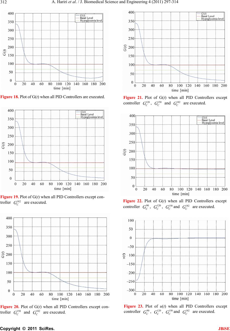

A. Hariri et al. / J. Biomedical Science and Engineering 4 (2011) 297-314 312
Figure 18. Plot of G(t) when all PID Controllers are executed.
Figure 19. Plot of G(t) when all PID Controllers except con-
troller 182
C
G are executed.
Figure 20. Plot of G(t) when all PID Controllers except con-
troller 150
C
G and 182
C
G are executed.
Figure 21. Plot of G(t) when all PID Controllers except
controller 120
C
G, 150
C
G and 182
C
G are executed.
Figure 22. Plot of G(t) when all PID Controllers except
controller 90
C
G, 120
C
G, 150
C
Gand 182
C
G are executed.
Figure 23. Plot of u(t) when all PID Controllers except
controller 90
C
G, 120
C
G, 150
C
Gand 182
C
G are executed.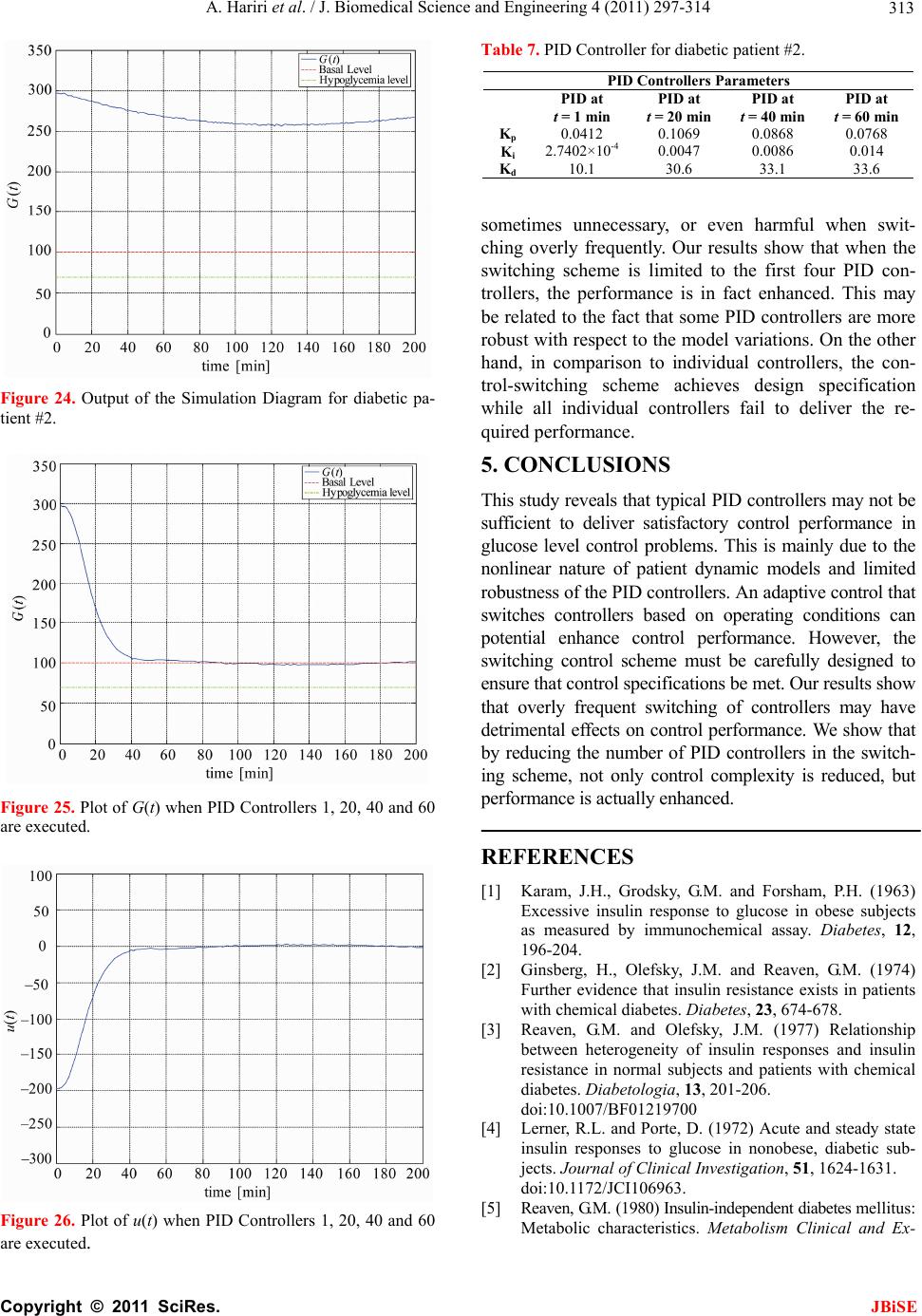

A. Hariri et al. / J. Biomedical Science and Engineering 4 (2011) 297-314 313
Figure 24. Output of the Simulation Diagram for diabetic pa-
tient #2.
Figure 25. Plot of G(t) when PID Controllers 1, 20, 40 and 60
are executed.
Figure 26. Plot of u(t) when PID Controllers 1, 20, 40 and 60
are executed.
Table 7. PID Controller for diabetic patient #2.
PID Controllers Parameters
PID at
t = 1 min PID at t = 20 min PID at t = 40 min PID at t = 60 min
Kp 0.0412 0.1069 0.0868 0.0768
Ki 2.7402×10-4 0.0047 0.0086 0.014
Kd 10.1 30.6 33.1 33.6
sometimes unnecessary, or even harmful when swit-
ching overly frequently. Our results show that when the
switching scheme is limited to the first four PID con-
trollers, the performance is in fact enhanced. This may
be related to the fact that some PID controllers are more
robust with respect to the model variations. On the other
hand, in comparison to individual controllers, the con-
trol-switching scheme achieves design specification
while all individual controllers fail to deliver the re-
quired performance.
5. CONCLUSIONS
This study reveals that typical PID controllers may not be
sufficient to deliver satisfactory control performance in
glucose level control problems. This is mainly due to the
nonlinear nature of patient dynamic models and limited
robustness of the PID controllers. An adaptive control that
switches controllers based on operating conditions can
potential enhance control performance. However, the
switching control scheme must be carefully designed to
ensure that control specifications be met. Our results show
that overly frequent switching of controllers may have
detrimental effects on control performance. We show that
by reducing the number of PID controllers in the switch-
ing scheme, not only control complexity is reduced, but
performance is actually enhanced.
REFERENCES
[1] Karam, J.H., Grodsky, G.M. and Forsham, P.H. (1963)
Excessive insulin response to glucose in obese subjects
as measured by immunochemical assay. Diabetes, 12,
196-204.
[2] Ginsberg, H., Olefsky, J.M. and Reaven, G.M. (1974)
Further evidence that insulin resistance exists in patients
with chemical diabetes. Diabetes, 23, 674-678.
[3] Reaven, G.M. and Olefsky, J.M. (1977) Relationship
between heterogeneity of insulin responses and insulin
resistance in normal subjects and patients with chemical
diabetes. Diabetologia, 13, 201-206.
doi:10.1007/BF01219700
[4] Lerner, R.L. and Porte, D. (1972) Acute and steady state
insulin responses to glucose in nonobese, diabetic sub-
jects. Journal of Clinical Investigation, 51, 1624-1631.
doi:10.1172/JCI106963.
[5] Reaven, G.M. (1980) Insulin-independent diabetes mellitus:
Metabolic characteristics. Metabolism Clinical and Ex-

A. Hariri et al. / J. Biomedical Science and Engineering 4 (2011) 297-314 314
perimental, 29, 445-454.
doi:10.1016/0026-0495(80)90170-5
[6] Bergman, R.N. and Cobelli, C. (1980) Minimal modeling,
partition analysis, and the estimation of insulin sensitivity.
Federation Proceedings, 39, 110-115.
[7] Shen, S-W., Reaven, G.M. and Farquhar, J.W. (1970)
Comparison of impedance to insulin-mediated glucose
uptake in normal and diabetic subjects. Journal of Clini-
cal Investigation, 49, 2151-2160.
doi:10.1172/JCI106433.
[8] Bergman, R.N., Ider, Y.Z., Bowden, C.R. and Cobelli, C.
(1979) Quantitative estimation of insulin sensitivity. Ameri-
can Journal of Physiology, 236, E667-E677.
[9] Pacini, G. and Bergman, R.N. (1986) MINMOD, A
computer program to calculate insulin and pancreatic re-
sponsivity from the frequently sampled intravenous glu-
cose tolerance test. Computer Methods and Programs in
Biomedicine, 23, 113-122
[10] Bergman, R.N., Phillips, L.S. and Cobelli, C. (1981)
Physiologic evaluation of factors controlling glucose tol-
erance in man, measurement of insulin sensitivity and
-cell glucose sensitivity from the response to intrave-
nous glucose. Journal of Clinical Investigation, 68, 1456
-1467. doi:10.1172/JCI110398
[11] Bergman, R.N. and Urquhart, J. (1971) The pilot gland
approach to the study of insulin secretory dynamics. Re-
cent Progress in Hormone Research, 27, 583-605.
[12] Nomura, M., Shichiri, M., Kawamori, R., Yamasaki, Y.,
Iwama, N. and Abe, H. (1984) A mathematical insulin-
secretion model and its validation in isolated rat pancre-
atic islets perifusion. Computers and Biomedical Re-
search, 17, 570-579.
doi:10.1016/0010-4809(84)90021-1
[13] Buchanan, T.A., Metzger, B.E., Freinkel, N. and Berg-
man, R.N. (1990) Insulin sensitivity and B-cell respon-
siveness to glucose during late pregnancy in lean and
moderately obese women with normal glucose tolerance
or mild gestational diabetes. American Journal of Ob-
stetrics and Gynecology, 162, 1008-1014.
[14] Lynch, S.M. and Bequette, B.W. (2001) Estimation-based
model predictive control of blood glucose in type i dia-
betics: A simulation study. IEEE Transations on Bio-
medical Engineering conferences, 79-80.
[15] Fisher, M.E. (1991) A semi-closed loop algorithm for the
control of blood glucose levels in diabetes. IEEE Transa-
tions on Biomedical Engineering conferences, 57-61.
[16] Furler, S.M., Kraegen, E.W., Bell, D.J., Smallwood, R.H.,
and Chisolm, D.J. (1985) Blood glucose control by in-
termittent loop closure in the basal mode: Computer
simulation studies with a diabetic model. Diabetes Care,
8, 553-561.
[17] Ibbini, M.S., Masadeh, M.A. and Amer, M.M.B. (2004)
A semiclosed-loop optimal control system for blood glu-
cose level in diabetics. Journal of Medical Engineering
& Technology, 28, 189-196.
doi:10.1080/03091900410001662332.
[18] Furler, S.M., Kraegen, E.W., Smallwood, R.H. and
Chisholm, D.J. (1985) Blood glucose control by inter-
mittent loop closure in the basal mode: computer simula-
tion studies with a diabetic model. Diabetes Care, 8, 553-
561. doi:10.2337/diacare.8.6.553
[19] Insel, P.A., Liljenquist, J.E., Tobin, J.D., Sherwin, R.S.,
Watkins, P., Andres, R. and Berman, M. (1975) Insulin
control of glucose metabolism in man. Journal of Clini-
cal Investigation, 55, 1057-1066.
doi:10.1172/JCI108006
[20] Grodsky, G.M. (1972) A threshold distribution hypothesis
for packet storage of insulin and its mathematical mod-
eling. Journal of Clinical Investigation, 51, 2047-2059.
doi:10.1172/JCI107011
[21] Sherwin, R.S., Kramer, K.J., Tobin, J.D., Insel, P.A.,
Liljenquist, J.E., Berman, M. and Andres, R. (1974) A
model of the kinetics of insulin in man. Journal of Clini-
cal Investigation, 53, 1481-1492.
[22] Turner, R.C., Holman, R.R., Mathews, D., Hockaday,
T.D.R. and Peto, J. (1979) Insulin deficiency and insulin
resistance interaction in diabetes: Estimation of their
relative contribution by feedback analysis from basal in-
sulin and glucose concentrations. Metabolism Clinical
and Experimental, 28, 1086-1096.
doi:10.1016/0026-0495(79)90146-X
[23] Lerner, R.L. and Porte, D. (1971) Relationships between
intravenous glucose loads, insulin responses and glucose
disappearance rate. Journal of Clinical Endocrinology &
Metabolism, 33, 409-417
[24] Bolie, V.W. (1961) Coefficients of normal blood glucose
regulation. Journal of Applied Physiology, 16, 783-788.
[25] Guyton, A.C. and Hall, J.E. (1996) Text book of medical
physiology, 9th Edition, Saunders.
[26] The American Diabetes Association is a US leading non-
profit health organization providing diabetes research,
information and advocacy since 1940.
[27] Gaetano, A.D. and Arino, O. (2000) Mathematical mod-
eling of the intravenous glucose tolerance test. Journal of
Mathematical Biology, 40, 136-168.
doi:10.1007/s002850050007
[28] Marquardt, D.W. (1963) An algorithm for least-squares
estimation of non-linear parameters. Journal of the Soci-
ety for Industrial and Applied Mathematics, 11, 431-441.
doi:10.1137/0111030
[29] Goodwin, C. and Payne, R.L. (1977) Dynamic System
Identification. Academic Press, Inc., New York.
[30] Lourakis, M. (2005) A brief description of the leven-
berg-marquardt algorithm implemented by levmar. Insti-
tute of Computer Science, Foundation for Research and
Technology.
[31] De Groot, M.H. and Schervish, M.J. (2002) Probability
and statistics. 3rd Edition, MA: Addison-Wesley, Boston.