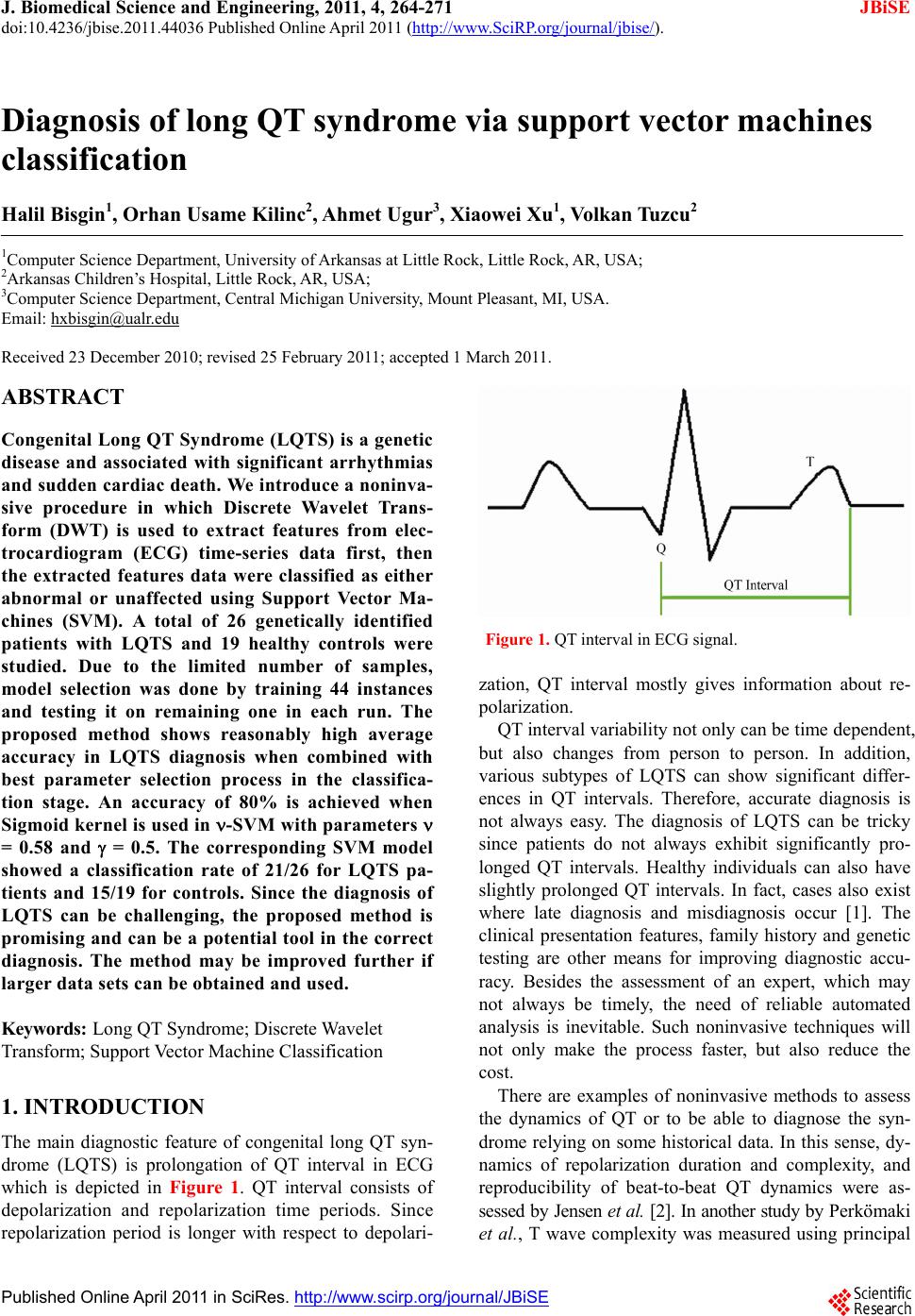J. Biomedical Science and Engineering, 2011, 4, 264-271 JBiSE
doi:10.4236/jbise.2011.44036 Published Online April 2011 (http://www.SciRP.org/journal/jbise/).
Published Online April 2011 in SciRes. http://www.scirp.org/journal/JBiSE
Diagnosis of long QT syndrome via support vector machines
classification
Halil Bisgin1, Orhan Usame Kilinc2, Ahmet Ugur3, Xiaowei Xu1, Volkan Tuzcu2
1Computer Science Department, University of Arkansas at Little Rock, Little Rock, AR, USA;
2Arkansas Children’s Hospital, Little Rock, AR, USA;
3Computer Science Department, Central Michigan University, Mount Pleasant, MI, USA.
Received 23 December 2010; revised 25 February 2011; accepted 1 March 2011.
ABSTRACT
Congenital Long QT Syndrome (LQTS) is a genetic
disease and associated with significant arrhythmias
and sudden cardia c death. We introduce a noninva-
sive procedure in which Discrete Wavelet Trans-
form (DWT) is used to extract features from elec-
trocardiogram (ECG) time-series data first, then
the extracted features data were classified as either
abnormal or unaffected using Support Vector Ma-
chines (SVM). A total of 26 genetically identified
patients with LQTS and 19 healthy controls were
studied. Due to the limited number of samples,
model selection was done by training 44 instances
and testing it on remaining one in each run. The
proposed method shows reasonably high average
accuracy in LQTS diagnosis when combined with
best parameter selection process in the classifica-
tion stage. An accuracy of 80% is achieved when
Sigmoid kernel is used in -SVM with parameters 
= 0.58 and  = 0.5. The corresponding SVM model
showed a classification rate of 21/26 for LQTS pa-
tients and 15/19 for controls. Since the diagnosis of
LQTS can be challenging, the proposed method is
promising and can be a potential tool in the correct
diagnosis. The method may be improved further if
larger data sets can be obtained and used.
Keywords: Long QT Syndrome; Discrete Wavelet
Transform; Support Vector Machine Classification
1. INTRODUCTION
The main diagnostic feature of congenital long QT syn-
drome (LQTS) is prolongation of QT interval in ECG
which is depicted in Figure 1. QT interval consists of
depolarization and repolarization time periods. Since
repolarization period is longer with respect to depolari-
Figure 1. QT interval in ECG signal.
zation, QT interval mostly gives information about re-
polarization.
QT interval variability not only can be time dependent,
but also changes from person to person. In addition,
various subtypes of LQTS can show significant differ-
ences in QT intervals. Therefore, accurate diagnosis is
not always easy. The diagnosis of LQTS can be tricky
since patients do not always exhibit significantly pro-
longed QT intervals. Healthy individuals can also have
slightly prolonged QT intervals. In fact, cases also exist
where late diagnosis and misdiagnosis occur [1]. The
clinical presentation features, family history and genetic
testing are other means for improving diagnostic accu-
racy. Besides the assessment of an expert, which may
not always be timely, the need of reliable automated
analysis is inevitable. Such noninvasive techniques will
not only make the process faster, but also reduce the
cost.
There are examples of noninvasive methods to assess
the dynamics of QT or to be able to diagnose the syn-
drome relying on some historical data. In this sense, dy-
namics of repolarization duration and complexity, and
reproducibility of beat-to-beat QT dynamics were as-
sessed by Jensen et al. [2]. In another study by Perkömaki
et al., T wave complexity was measured using principal

H. Bisgin et al. / J. Biomedical Science and Engineering 4 (2011) 264-271 265
component analysis [3]. They have shown that QT vari-
ability, mean T wave complexity, and T wave complex-
ity variability helped in distinguishing patients from
healthy controls.
Studies based on wavelet transform also helped to
figureout some hidden patterns within the ECG signals.
Couderc et al. pointed out how wavelet transform is a
promising way of analyzing ECG signals [4]. From ECG
pattern recognition to analysis of ventricular repolariza-
tion, wavelet transform is considered as a technique that
can highlight details of ECG signals in noninvasive
electrocardiology. QRS detection via wavelet analysis by
Li is a prominent example [5].
In order to analyze QT interval time frequency, Wong
et al. employed DWT on a data set which consisted of
exercise ECG signals [6]. They demonstrated that their
QT interval automatic measurement methodology was
very similar to clinical observations. Strachan et al. de-
veloped a Hidden Markovian Model (HMM) based QT
analysis method [7]. Specifically, they trained wave-
forms from ECG signals via wavelet transform which
were already annotated by the experts. They used a large
data set in order to train for HMM for automated QT
analysis.
Besides signal processing tools, other statistical learning
mechanisms may help to identify pathological cases ap-
propriately. In this study, we utilize both signal process-
ing method DWT and statistical learning procedure
SVM. The outline of the paper is as follows. In Section 2,
we describe the methods that we have use throughout the
study including DWT, feature extraction with DWT, and
formulation n of SVM with its variations. In Section 3,
we explain data preprocessing and the grid search
mechanism to find the best parameters. In Section 4, we
discuss the results and present our conclusions.
2. METHODS
2.1. Discr ete Wavelet Transform
Human perception or any other techniques in time do-
main cannot always capture some critical details in the
signal. For example, although ECG signals seem to be
very similar to each other, a physician is not always able
to diagnose a pathological case without using further
analyses. Especially, non-stationary signals are hard to
analyze even with Fourier transformation (FT) in fre-
quency domain. It is because Fourier representation of a
time domain signal lacks time resolution. Moreover, FT
can only give global information about the frequency
distribution of a signal. On the other hand, wavelet
transformation is capable of transforming a signal in a
multi-resolutionary pattern. Due to its multi-resolution
property, it can also provide an analysis of the signal at
different frequencies with different resolutions rather
than a global knowledge [8].
In order to attain the characteristics of any signal in
the frequency domain, the signal is expressed in terms of
basis functions. Since these functions form a basis for
the original signal x(t), they need to be orthogonal. FT of
x(t) consists of cosine and sine functions, whereas
wavelet transform is a linear combination of orthonor-
mal functions, wavelets [9]. Being orthonormal requires
unity in terms of length besides orthogonality. Haar
wavelet is one of the well-known functions which is also
adopted in the present study. The Haar wavelet can be
described as:

10 12
112 1(1)
0
t
tt
otherwise




 



After determining the mother wavelet,
 (t), its varia-
tions ,
1
ba tb
a
a




 are generated to form the
basis. Here


,ab 


are said to be translation
and scale parameters.
Translation refers to shifting over time that enables us
observe the time resolution. Resolution in terms of fre-
quency is also achieved by scale parameter [9].
A dyadic transform makes it more convenient to ma-
nipulate the wavelet to generate basis functions. In other
words, if we take a = 2–j and b = k2–j, the following re-
cursive function represents a set of functions or bases
[9].


2
,22
jj
jk ttk

 
(2)
Hence any signal x(t) can be expressed by the series


2
,
,
22
jj
jk
jk
x
ta tk




(3)
Eq.3 can be simplified as


,,
,
jk jk
jk
x
ta t

 (4)
Both Eqs. 3 and 4 imply that aj,k are the coefficients of
base functions 
j,k (t) as we discussed earlier. Since we
have an orthonormal basis, it’s clear that any coefficient
aj,k can be derived from the inner product, < 
j,k (t), x(t)
>. The two-dimensional set of coefficients, aj,k, are said
to be DWT of x(t) [9].
In the light of the definition of DWT, it’s worth to
state that equation 4 can be also written as


,,
,
,
jk jk
jk
x
ttxtt


(5)
Referring to the wavelet, shifting over the time and
variation of the scale contribute to time-scale representa-
tion of a signal. In discrete case, the above analysis is

H. Bisgin et al. / J. Biomedical Science and Engineering 4 (2011) 264-271 266
achieved in a way that the signal is passed through com-
bined high-pass and low-pass filters incorporated with
subsampling [8]. If a signal is filtered by changing cut-
off frequencies in a cascaded filter model, a frequency
resolution (scale in wavelet terminology) is obtained.
Subsampling is applied to attain the resolution over time.
That is to remove some samples from the signal. If a
signal is subsampled by 2, it is implied that every other
sample remains in the sequence.
The implementation of the idea above is done by a
digital filtering approach where the signal is filtered at
different cut-off frequencies at different scales. The
process is summarized as filter bank approach in the
literature [10]. At each level of the procedure, low-pass
and high-pass filters are employed to the signals which
are subsampled by 2. Output of the highpass filtered part
of the signal is processed based on the same principle. In
other words, the output becomes an input for the next
filter pair where cut-off is halved and subsampling oc-
curs again. This process continues until no subsampling
is possible [10].
If we let x[n], g[n] and h[n] be the signal, high pass
filter, and low pass filter respectively, the following
convolutions in Eqs.6 and 7 give us different representa-
tions from x[n]. Figure 2 shows the cascading filter
model for this iterative procedure.






2
high n
yk xngkn
 (6)






2
lown
yk xnhkn
 (7)
At the end of the iterative process, a series of coeffi-
cients, which come from the output of the low-pass fil-
ters at every level, is obtained. Due to the subsampling,
the number of coefficients decreases in log2 scale at each
stage. The concatenation all of the coefficients becomes
the DWT presentation of the signal, x[n] and yields the
same signal length.
2.2. Feature Extraction via DWT
Wu et al. show that DWT is more capable of capturing
the underlying shape of the original signal than Discrete
Fourier Transform (DFT) and DWT has less error of
distance estimates on the transformed domains than DFT
in its nature [11,12]. Therefore, in this study DWT is
preferred to extract features. However, coefficients ob-
tained at every level and the energy that those coeffi-
cients preserve can be considered as representing com-
ponents of the original signal. Mörchen compares dif-
ferent manipulations of those coefficients [13].
In this study, we have adopted the proposed method
by Wu. We have selected k largest coefficients since they
have the largest amount of the energy, which means that
these are the most representative. Instead of using just
Figure 2. Cascading filter design.
coefficients, energy contained by coefficients is taken
into account in an aggregated pattern. As Mörchen sug-
gests, ordered coefficients and their energies are accu-
mulated in  steps where we have 2 length signal
[13]. Emerging  partial sums are considered as fea-
tures of the input signal. Hence, in the classification
process, instead of the entire signal, we are able to do
our experiments with a very small representative data set.
This will not only decrease computational burden, but
also discard irrelevant information embedded in the sig-
nal [13].
2.3. Support Vector Machine Classification
Linear models such as linear regression, logistic regres-
sion as well as perceptron algorithm for linear classifica-
tion are the most prominent ones that can be used for
classification when all the attributes are numeric. How-
ever, their ability to draw boundaries between two
classes is restricted to some point. Specifically, for many
practical problems, they become too simple in handling
a complicated data set. On the other hand, SVM over-
comes such problems using also linear models, but in a
higher dimensional space. It behaves as if it handles a
linear case; therefore, its capability of putting non-linear
boundaries is possible [14].
If we assume a two-class case, we are supposed to
find a hyperplane which divides our data set into two
parts accordingly. Many times, it is possible to find more
than one boundary to partition the set. The question is to
find the best division. This is simply an optimization
problem. In other words, one has to find most appropri-
ate border via maximizing distances from each set to the
separating hyperplane. Actually, the goal of employing
SVM is to determine the separating boundary with the
maximum margin [15].
Let
 


1
,,1,1
n
p
ii iii
Dxyx y  where xi is a
p-dimensional vector and yi’s are the class labels. If we
define a hyperplane H for set D, we have:
T
T
11
11
i
i
bify
bify




wx
wx (8)
Then, our aim is to maximize the distance2  
w,
which is also depicted in the Figur e 3.

H. Bisgin et al. / J. Biomedical Science and Engineering 4 (2011) 264-271 267
Figure 3. Margin to be maximized.
In order to maximize 2  
w, it is obvious that the
denominator needs to be minimized. One approach to
solve this problem is to define

T
1
2
  www which
exactly fits to the quadratic programming approach [15].
More formally, our primal form is as follows:


T
T
1
min 2
such that
1
ii
yb



 www
wx
(9)
where w and b are design variables. If we rewrite our
model in a dual form where we have Lagrange multiplier

i for each constraint in the primal form, we obtain the
following model:
T
1
max 2
such that
0, 0
iijijij
iii
yy
y






xx
(10)
Then we derive that iii
y
  wx
and T
kk
bywx
for any k x such that 0
k

. As a matter of fact, xk
values which correspond to 0
k

 are called support
vectors [15]. Those data points are the ones which con-
stitute the classification function

fx. Namely, if we
suppose that x is a test point and we are supposed to de-
termine a label for it, we simply plug it into the follow-
ing:

T
iii
f
yb

 xxx (11)
In a non-separable linear case, we have a regulariza-
tion parameter C in the presence of slack variables 
i
which helps to manage the misclassification and the
noise. Slightly modified optimization problem turns out
to be in primal form like:


T
T
1
min 2
such that
1and 0
i
iii i
C
yb


 



www
wx
(12)
That implies the dual form is going to be
T
1
max 2
such that
0, 0
iijijij
iii
yy
Cy

 




xx
(13)
where slack variables do not exist anymore. Since C is a
regularization parameter, it prevents from any over fit-
ting problem. We will refer to this kind of procedure as
C-Support Vector Machine classification (C-SVM). The
trade off between minimizing the training error and the
maximizing the margin is managed by the constant C
[15]. Since there is no way of determining it a priori, n
-Support Vector Machine classification (n-SVM) was
introduced by Schölkopf and Smola [16]. Optimization
procedure was changed in a way that parameter C was
removed while a new parameter, n was introduced. This
modification aims to control not only the number of
margin errors by n, but also the number of support vec-
tors. The new formulation in terms of dual problem is as
follows:
T
11
1
max 2
such that
1
0, 0,
mm
ijiji j
ij
iiii
yy
y
m















xx
(14)
In the case of non-separable data set, kernel functions


:  xx
are used to map the data points into a
higher dimensional space where the set is not non-sepa-
rable anymore. The inner product T
ij
xxin the optimiza-
tion problem above is replaced by a kernel function




T
,
ij i
K  xxx . We applied kernel trick with radial
basis and sigmoid functions, which are expressed below
respectively [15].


2
T
0
,e
(, )tanh
ij
ij
ij ij
K
K
a





xx
xx
xx xx
(15)
2.4. Model Validation
During training period it is possible to capture all the
details of the training set. However, obtained model may
not necessarily perform well on a testing set. As a matter
of fact, if the model tries to handle every data point in-
cluding the noise, overfitting may be a potential problem.
T1
ibwx T0
ibwx
T1
ibwx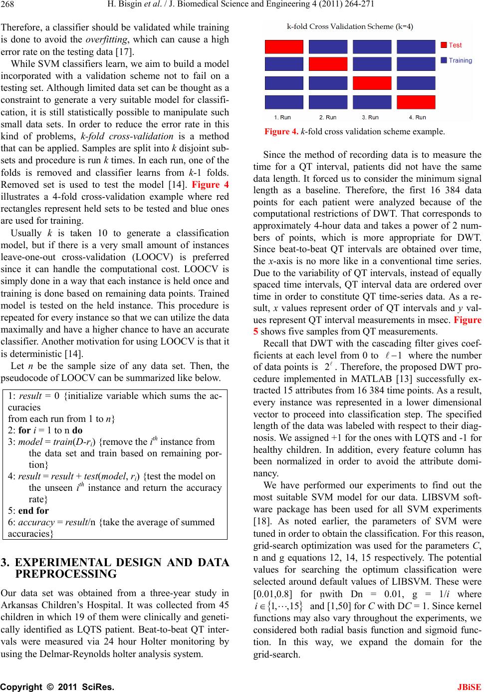


H. Bisgin et al. / J. Biomedical Science and Engineering 4 (2011) 264-271 268
Therefore, a classifier should be validated while training
is done to avoid the overfitting, which can cause a high
error rate on the testing data [17].
While SVM classifiers learn, we aim to build a model
incorporated with a validation scheme not to fail on a
testing set. Although limited data set can be thought as a
constraint to generate a very suitable model for classifi-
cation, it is still statistically possible to manipulate such
small data sets. In order to reduce the error rate in this
kind of problems, k-fold cross-validation is a method
that can be applied. Samples are split into k disjoint sub-
sets and procedure is run k times. In each run, one of the
folds is removed and classifier learns from k-1 folds.
Removed set is used to test the model [14]. Figure 4
illustrates a 4-fold cross-validation example where red
rectangles represent held sets to be tested and blue ones
are used for training.
Usually k is taken 10 to generate a classification
model, but if there is a very small amount of instances
leave-one-out cross-validation (LOOCV) is preferred
since it can handle the computational cost. LOOCV is
simply done in a way that each instance is held once and
training is done based on remaining data points. Trained
model is tested on the held instance. This procedure is
repeated for every instance so that we can utilize the data
maximally and have a higher chance to have an accurate
classifier. Another motivation for using LOOCV is that it
is deterministic [14].
Let n be the sample size of any data set. Then, the
pseudocode of LOOCV can be summarized like below.
1: res ult = 0 {initialize variable which sums the ac-
curacies
from each run from 1 to n}
2: for i = 1 to n do
3: model = train(D-ri) {remove the ith instance from
the data set and train based on remaining por-
tion}
4: re sul t = res ult + test(model, ri) {test the model on
the unseen ith instance and return the accuracy
rate}
5: end for
6: accuracy = re sult/n {take the average of summed
accuracies}
3. EXPERIMENTAL DESIGN AND DATA
PREPROCESSING
Our data set was obtained from a three-year study in
Arkansas Children’s Hospital. It was collected from 45
children in which 19 of them were clinically and geneti-
cally identified as LQTS patient. Beat-to-beat QT inter-
vals were measured via 24 hour Holter monitoring by
using the Delmar-Reynolds holter analysis system.
Figure 4. k-fold cross validation scheme example.
Since the method of recording data is to measure the
time for a QT interval, patients did not have the same
data length. It forced us to consider the minimum signal
length as a baseline. Therefore, the first 16 384 data
points for each patient were analyzed because of the
computational restrictions of DWT. That corresponds to
approximately 4-hour data and takes a power of 2 num-
bers of points, which is more appropriate for DWT.
Since beat-to-beat QT intervals are obtained over time,
the x-axis is no more like in a conventional time series.
Due to the variability of QT intervals, instead of equally
spaced time intervals, QT interval data are ordered over
time in order to constitute QT time-series data. As a re-
sult, x values represent order of QT intervals and y val-
ues represent QT interval measurements in msec. Figure
5 shows five samples from QT measurements.
Recall that DWT with the cascading filter gives coef-
ficients at each level from 0 to 1 where the number
of data points is 2. Therefore, the proposed DWT pro-
cedure implemented in MATLAB [13] successfully ex-
tracted 15 attributes from 16 384 time points. As a result,
every instance was represented in a lower dimensional
vector to proceed into classification step. The specified
length of the data was labeled with respect to their diag-
nosis. We assigned +1 for the ones with LQTS and -1 for
healthy children. In addition, every feature column has
been normalized in order to avoid the attribute domi-
nancy.
We have performed our experiments to find out the
most suitable SVM model for our data. LIBSVM soft-
ware package has been used for all SVM experiments
[18]. As noted earlier, the parameters of SVM were
tuned in order to obtain the classification. For this reason,
grid-search optimization was used for the parameters C,
n and g equations 12, 14, 15 respectively. The potential
values for searching the optimum classification were
selected around default values of LIBSVM. These were
[0.01,0.8] for nwith Dn = 0.01, g = 1/i where


1, ,15i and [1,50] for C with DC = 1. Since kernel
functions may also vary throughout the experiments, we
considered both radial basis function and sigmoid func-
tion. In this way, we expand the domain for the
grid-search.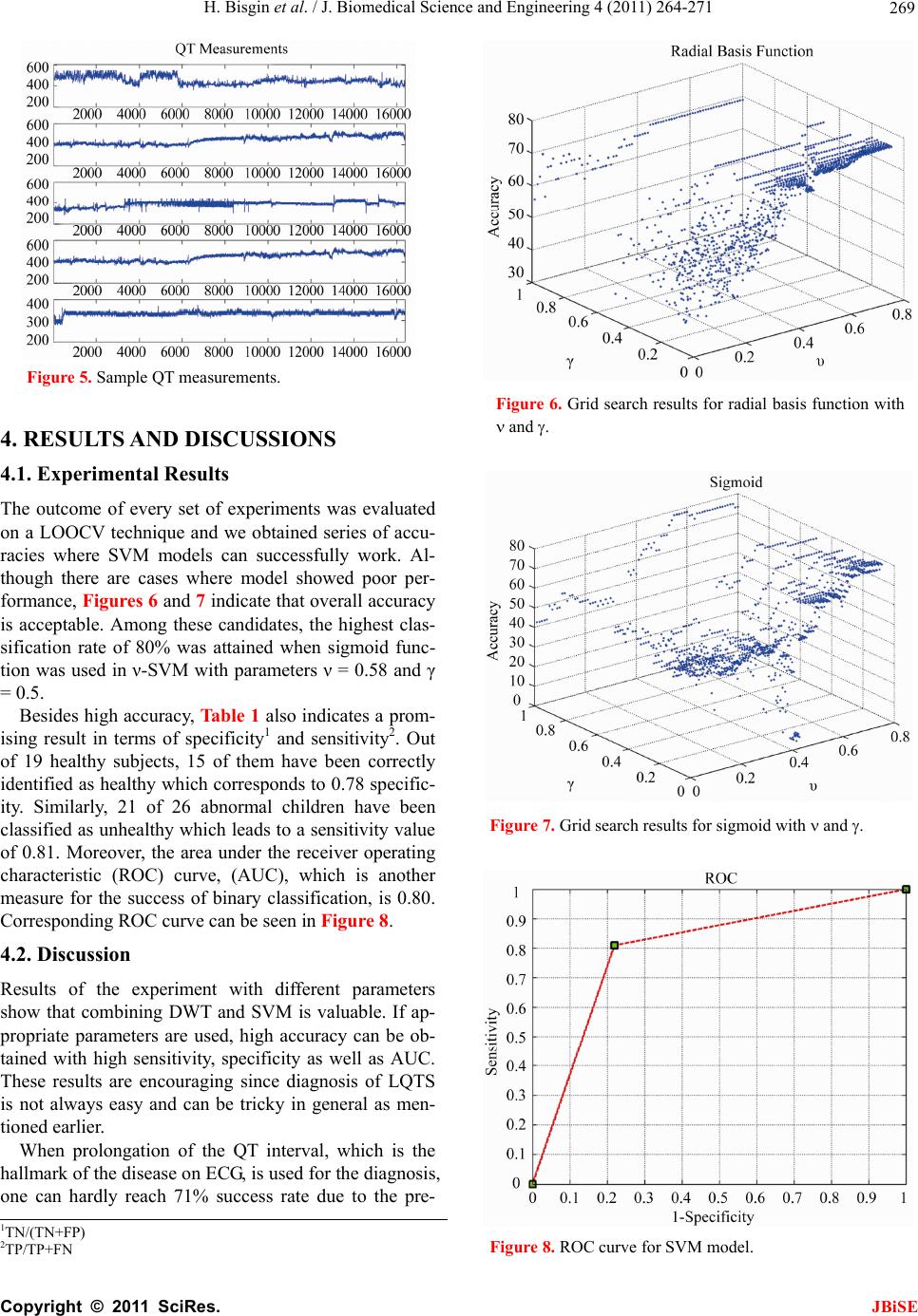

H. Bisgin et al. / J. Biomedical Science and Engineering 4 (2011) 264-271 269
Figure 5. Sample QT measurements.
4. RESULTS AND DISCUSSIONS
4.1. Experimental Results
The outcome of every set of experiments was evaluated
on a LOOCV technique and we obtained series of accu-
racies where SVM models can successfully work. Al-
though there are cases where model showed poor per-
formance, Figures 6 and 7 indicate that overall accuracy
is acceptable. Among these candidates, the highest clas-
sification rate of 80% was attained when sigmoid func-
tion was used in ν-SVM with parameters ν = 0.58 and γ
= 0.5.
Besides high accuracy, Table 1 also indicates a prom-
ising result in terms of specificity1 and sensitivity2. Out
of 19 healthy subjects, 15 of them have been correctly
identified as healthy which corresponds to 0.78 specific-
ity. Similarly, 21 of 26 abnormal children have been
classified as unhealthy which leads to a sensitivity value
of 0.81. Moreover, the area under the receiver operating
characteristic (ROC) curve, (AUC), which is another
measure for the success of binary classification, is 0.80.
Corresponding ROC curve can be seen in Figure 8.
4.2. Discussion
Results of the experiment with different parameters
show that combining DWT and SVM is valuable. If ap-
propriate parameters are used, high accuracy can be ob-
tained with high sensitivity, specificity as well as AUC.
These results are encouraging since diagnosis of LQTS
is not always easy and can be tricky in general as men-
tioned earlier.
When prolongation of the QT interval, which is the
hallmark of the disease on ECG, is used for the diagnosis,
one can hardly reach 71% success rate due to the pre-
Figure 6. Grid search results for radial basis function with
 and 

Figure 7. Grid search results for sigmoid with  and 

Figure 8. ROC curve for SVM model.
1TN/(TN+FP)
2TP/TP+FN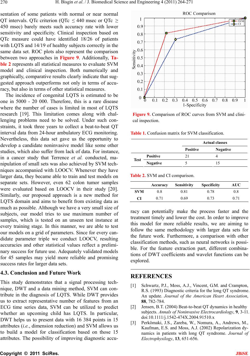

H. Bisgin et al. / J. Biomedical Science and Engineering 4 (2011) 264-271 270
sentation of some patients with normal or near normal
QT intervals. QTc criterion (QTc ≤ 440 msec or QTc ≥
450 msec) barely meets such accuracy rate with lower
sensitivity and specificity. Clinical inspection based on
QTc measure could have identified 18/26 of patients
with LQTS and 14/19 of healthy subjects correctly in the
same data set. ROC plots also represent the comparison
between two approaches in Figure 9. Additionally, Ta-
ble 2 represents all statistical measures to evaluate SVM
model and clinical inspection. Both numerically and
graphically, comparative results clearly indicate that sug-
gested approach outperforms not only in terms of accu-
racy, but also in terms of other statistical measures.
The incidence of congenital LQTS is estimated to be
one in 5000 - 20 000. Therefore, this is a rare disease
where the number of cases is limited in most of LQTS
research [19]. This limitation comes along with chal-
lenging problems need to be solved. Under such con-
straints, it took three years to collect a beat-to-beat QT
interval data from 24-hour ambulatory ECG monitoring.
Nevertheless, this data set gave us the opportunity to
develop a candidate noninvasive model like some other
studies, which also suffer from lack of data. For instance,
in a cancer study that Terrence et al. conducted, ma-
nipulation of small sets was also achieved by SVM tech-
niques accompanied with LOOCV. Whenever they have
larger data, they became able to train and test models on
separate sets. However, even 62 colon tumor samples
were evaluated based on LOOCV in their study [20].
Similarly, our proposed approach is a new method for
LQTS domain and aims to benefit from existing data as
much as possible. Although we have a very small size of
subjects, our model tries to use maximum number of
samples, which is tested on an unseen test instance at
every training stage. In this manner, we are able to test
our models on a grid of parameters. Since for every can-
didate parameter triple we conduct LOOCV, resulting
accuracies and other statistical values reflect a prelimi-
nary success for future use. Adequately validated models
for 45 samples may yield more reliable and promising
success rates for larger data sets.
4.3. Conclusion and Future Work
This study demonstrates that a signal processing tech-
nique, DWT and a data mining method, SVM can con-
tribute in the diagnosis of LQTS. While DWT provides
us to extract representative number of features from an
ECG time series data, SVM can be utilized to predict
whether an upcoming child has LQTS. In particular,
DWT helps us to present data with 16 384 points in 15
attributes (i.e., dimension reduction) and SVM allows us
to build a model for classification based on those 15
attributes. The possibility of improving diagnostic accu-
Figure 9. Comparison of ROC curves from SVM and clini-
cal inspection.
Table 1. Confusion matrix for SVM classification.
Actual classes
Positive Negative
Positive 21 4
Test Negative 5 15
Table 2. SVM and CI comparison.
Accuracy Sensitivity Specificity AUC
SVM 0.8 0.81 0.78 0.8
CI 0.71 0.69 0.73 0.71
racy can potentially make the process faster and the
treatment timely and lower the cost. In order to improve
this model for more reliable results, we are aiming to
follow the same methodology with larger data sets for
the future work. Furthermore, a comparison with other
classification methods, such as neural networks is possi-
ble. For the feature extraction part, different combina-
tions of DWT coefficients and wavelet functions can be
explored.
REFERENCES
[1] Schwartz, P.J., Moss, A.J., Vincent, G.M. and Crampton,
R.S. (1993) Diagnostic criteria for the long QT syndrome.
An update. Journal of the American Heart Association,
88, 782-784.
[2] Jensen, B.T. (2004) Beat-to-beat QT dynamics in healthy
subjects. Annals of Noninvasive Electrocardiology, 9, 3-11.
doi:10.1111/j.1542-474X.2004.91510.x
[3] Perkömaki, J.S., Zareba, W., Nomura, A., Andrews, M.,
Kaufman, E.S. and Moss, A.J. (2002) Repolarization dy-
namics in patients with long QT syndrome. Journal of
Electrophysilogy, 13, 651-656.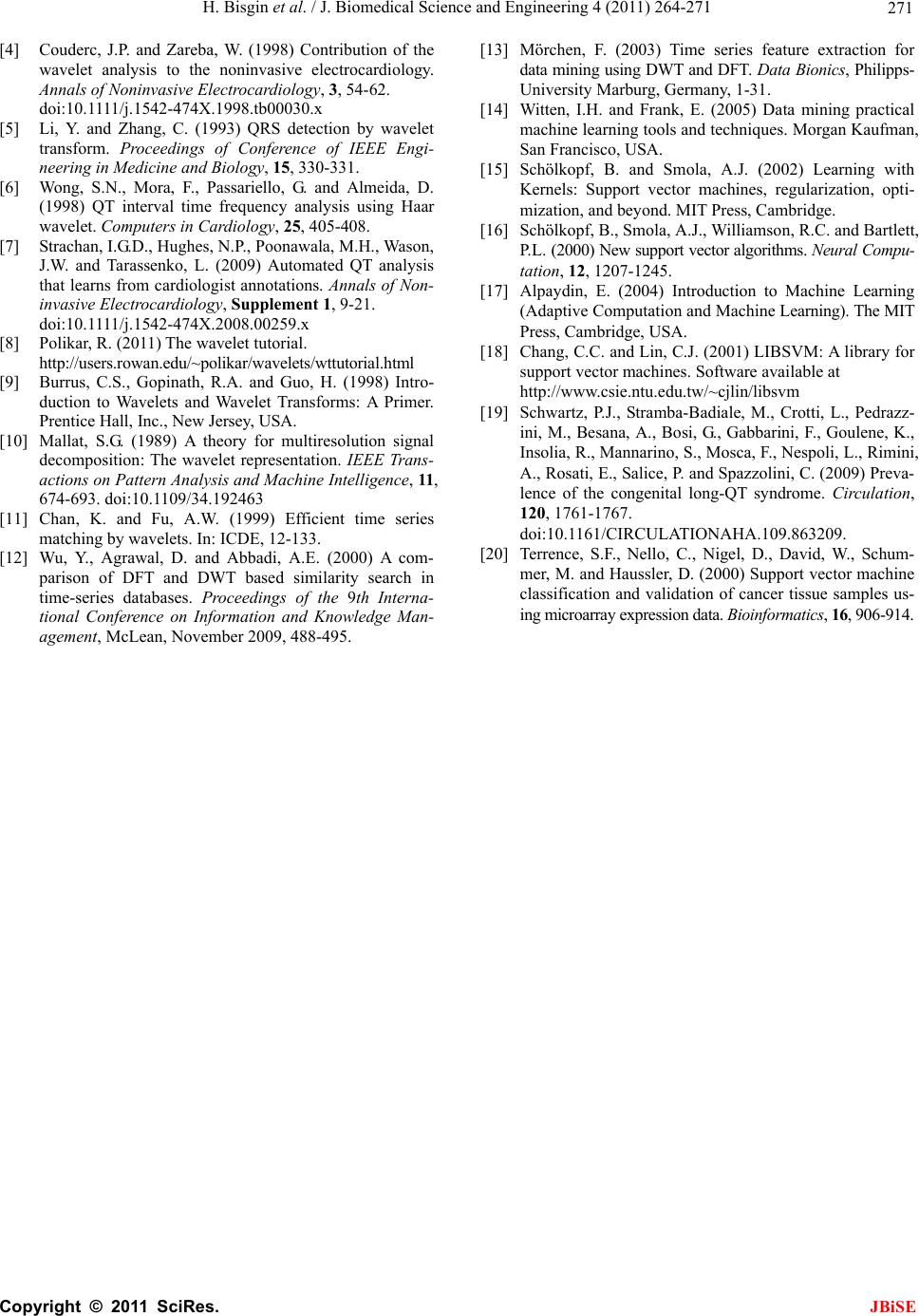

H. Bisgin et al. / J. Biomedical Science and Engineering 4 (2011) 264-271 271
[4] Couderc, J.P. and Zareba, W. (1998) Contribution of the
wavelet analysis to the noninvasive electrocardiology.
Annals of Noninvasive Electrocardiology, 3, 54-62.
doi:10.1111/j.1542-474X.1998.tb00030.x
[5] Li, Y. and Zhang, C. (1993) QRS detection by wavelet
transform. Proceedings of Conference of IEEE Engi-
neering in Medicine and Biology, 15, 330-331.
[6] Wong, S.N., Mora, F., Passariello, G. and Almeida, D.
(1998) QT interval time frequency analysis using Haar
wavelet. Computers in Cardiology, 25, 405-408.
[7] Strachan, I.G.D., Hughes, N.P., Poonawala, M.H., Wason,
J.W. and Tarassenko, L. (2009) Automated QT analysis
that learns from cardiologist annotations. Annals of Non-
invasive Electrocardiology, Supplement 1, 9-21.
doi:10.1111/j.1542-474X.2008.00259.x
[8] Polikar, R. (2011) The wavelet tutorial.
http://users.rowan.edu/~polikar/wavelets/wttutorial.html
[9] Burrus, C.S., Gopinath, R.A. and Guo, H. (1998) Intro-
duction to Wavelets and Wavelet Transforms: A Primer.
Prentice Hall, Inc., New Jersey, USA.
[10] Mallat, S.G. (1989) A theory for multiresolution signal
decomposition: The wavelet representation. IEEE Trans-
actions on Pattern Analysis and Machine Intelligence, 11,
674-693. doi:10.1109/34.192463
[11] Chan, K. and Fu, A.W. (1999) Efficient time series
matching by wavelets. In: ICDE, 12-133.
[12] Wu, Y., Agrawal, D. and Abbadi, A.E. (2000) A com-
parison of DFT and DWT based similarity search in
time-series databases. Proceedings of the 9th Interna-
tional Conference on Information and Knowledge Man-
agement, McLean, November 2009, 488-495.
[13] Mörchen, F. (2003) Time series feature extraction for
data mining using DWT and DFT. Data Bionics, Philipps-
University Marburg, Germany, 1-31.
[14] Witten, I.H. and Frank, E. (2005) Data mining practical
machine learning tools and techniques. Morgan Kaufman,
San Francisco, USA.
[15] Schölkopf, B. and Smola, A.J. (2002) Learning with
Kernels: Support vector machines, regularization, opti-
mization, and beyond. MIT Press, Cambridge.
[16] Schölkopf, B., Smola, A.J., Williamson, R.C. and Bartlett,
P.L. (2000) New support vector algorithms. Neural Compu-
tation, 12, 1207-1245.
[17] Alpaydin, E. (2004) Introduction to Machine Learning
(Adaptive Computation and Machine Learning). The MIT
Press, Cambridge, USA.
[18] Chang, C.C. and Lin, C.J. (2001) LIBSVM: A library for
support vector machines. Software available at
http://www.csie.ntu.edu.tw/~cjlin/libsvm
[19] Schwartz, P.J., Stramba-Badiale, M., Crotti, L., Pedrazz-
ini, M., Besana, A., Bosi, G., Gabbarini, F., Goulene, K.,
Insolia, R., Mannarino, S., Mosca, F., Nespoli, L., Rimini,
A., Rosati, E., Salice, P. and Spazzolini, C. (2009) Preva-
lence of the congenital long-QT syndrome. Circulation,
120, 1761-1767.
doi:10.1161/CIRCULATIONAHA.109.863209.
[20] Terrence, S.F., Nello, C., Nigel, D., David, W., Schum-
mer, M. and Haussler, D. (2000) Support vector machine
classification and validation of cancer tissue samples us-
ing microarray expression data. Bioinformati cs, 16, 906-914.