Journal of Geoscience and Environment Protection, 2014, 2, 135-143
Published Online June 2014 in SciRes. http://www.scirp.org/journal/gep
http://dx.doi.org/10.4236/gep.2014.23018
How to cite this paper: Bogdanowicz, E. et al. (2014). Flood Risk for Embanked Rivers. Journal of Geoscience and Environ-
ment Protection, 2, 135-143. http://dx.doi.org/10.4236/gep.2014.23018
Flood Risk for Embanked Rivers
Ewa Bogdanowicz1, Witold G. Strupczewski2, Krzysztof Kochanek2, Iwona Markiewicz2
1Institute of Meteorology and Water Management, Podleśna 61, 01-673 Warsaw, Poland
2Institute of Geophysics, Polish Academy of Sciences, Księcia Janusza 64, 01-452 Warsaw, Poland
Received April 2014
Abstract
Flood frequency analysis (FFA) concentrates on peak flows of flood hydrographs. However, floods
that last years devastated large parts of Poland lead us to revision of the views on the assessment
of flood risk in Poland. It turned out that it is the prolonged exposure to high water on levees that
causes floods, not only the water overflowing the levee crest. This is because, the levees are
weakened by water and their disruption occurs when it seems that the danger is over, i.e. after
passing culmination. Two main causes of inundation of embanked rivers, namely over-crest flow
and wash out of the levees, are combined to assess the total risk of inundation. Therefore the risk
of inundation is the total of risk of exceeding embankment crest by flood peak and risk of washout
of levees. Hence, while modeling the flood events in addition to the maximum flow one should
consider also the duration of high water in a river channel, Analysis of the frequency of annual
peak flows based on annual maxima and peaks over threshold is the subject of countless publica-
tions. Therefore we will here mainly modeling the duration of high water levels. In the paper the
two-component model of flood hydrograph shape i.e. “duration of flooding-discharge- probability
of nonexceedance ” (DqF), with the methodology of its parameters estimation for sta- tionary case
was developed as a completion to the classical FFA with possible extension to non stationary flood
regime. The model combined with the technical evaluation of probability of levees breach due to
the d-days duration of flow above alarm stage gives the annual probability of inundation caused
by the embankment breaking. The results of theoretical research were supplemented by a practi-
cal example of the model application to the series for daily flow in the Vistula River in Szczucin.
Regardless promising results, this method is still in its infancy despite its great cognitive potential
and practical importance. Therefore, we would like to point to the usefulness and necessity of the
DqF models to the one-dimensional analysis of the peak flood hydrographs and to flood risk
analysis. This approach constitutes a new direction in FFA for embanked rivers.
Keywords
Flood Frequency Analy sis, Levee Break, Flood Duration, Maximum Likelihood, Nonstationarity
1. Introduction
The most popular way of flood protection in Poland is the embankment of the rivers. In consequence of this
passive way of protection, floods in Poland occur mostly due to the levee breach or very rarely to flow over the

E. Bogdanowicz et al.
136
crest of dikes. Sense of security in floodplains of embanked rivers results from the belief that levees protect
against the flood magnitude for which they were designed. So it creates the illusion that if the actual forecasted
flood peak does not exceed the safety levels related to levee’s designed value one can assume that the risk of
water overtopping the dike crest is negligible and so is the risk of flooding in the protected area. The records of
floods in Poland show that this is not true; more often the floods are the result of the prolonged exposure to high
water on levees. The levees are weakened by water and their disruption occurs when it seems that the danger is
over, i.e. after passing culmination. This is particularly dangerous because when the staff responsible for flood
protection and local residents breathe sigh of relief the worst is yet to come.
Therefore, apart from the magnitude of the peak flows another important factor should be taken into
consideration, i.e. the persistence of flood described by duration of high water levels. Long-lasting high stages
may weaken the levees’ structure (soaking) and cause dangerous leaks, blurs and breaks that threaten their
destruction. That is why the classical flood frequency analysis (FFA) concerning only the frequency of the
annual maximum (AM) flows (Bogdanowicz et al., 2011) is not suitable in this case and ought to be
supplemented by the analysis of the duration of flows over the given threshold. The joint risk of inundation
making allowance for the two main sources of vulnerability to flood hazard for areas protected by embankments,
i.e. over-crest flow and levees failure, has been proposed and defined.
In Poland, as in many other countries for each hydrological station two benchmark water levels, named the
warning stage and the alarm stage, have been specified. Although warning and alarm stages are assigned to the
places where water levels are observed, i.e. to the hydrological stations, their determination procedures as well
as other inundation risk characteristics take into account, inter alia, the elevation of the embankment system for
the whole adjacent river reach. So, the results of below analysis refer to the river reaches represented by data
observed at hydrological stations. The frequency of annual maximum uninterrupted duration, D (in days), of
flows over the flood alarm stage (Figure 1) can be used to assess the risk of flooding due to waning of the
levees' strength. The aim of this study is to introduce formal aspects of the Duration-flow-Frequency (DqF)
modelling in stationary and non-stationary conditions, to use it to assess the inundation risk due to the levees
breach and to combine it with the AM flow model to get the cumulative probability of inundation.
To cater for the conventional FFA, the flow discharge (QA) corresponding to the alarm stage (HA) is used
here, i.e. the upper limb of the rating curve is regarded as time invariant. The frequency of annual maximum
uninterrupted duration of flows, D (in hours, days, etc.), over the flood alarm stage (HA) (or equivalently over
the alarm flow (QA)) but excluding floods pouring over the embankment crest (which corresponds to flows
exceeding the overtopping flow QB) serves to assess the inundation risk of flood spilling out of river channel
caused by scouring the levees (Figure 2). Therefore, the dt = 0 in the [d] time-series denotes that the QA has not
been exceeded during the t-thyear (Qmax(t) < QA) or that the peak flow has exceeded the overtopping flow
(Qmax(t) > QB) where Qmax denotes the annual maximum discharge. Note that if more than one flood appears
in a year, the D and the annual peak flow (Qmax) can correspond to different floods (Figure 1). In the presented
statistical model, the duration (D) is considered as a random variable while the alarm flow discharge (QA) is the
fixed value.
The paper is built as follows: in the second section the concept of the inundation risk for embanked river is
defined. Then the Duration-Flow discharge-Frequency (DqF) model is introduced and estimations of its
parameter for stationary and non-stationary case are described and discussed. Taking into account the embank-
ment resistance, the annual probability of inundation caused by levees breaching is introduced. To illustrate the
proposed way of inundation risk assessment the case study for the Szczucin gauging station at the Vistula River
(Southern Poland) is presented (Section 4). The probability of inundation due to levees breaching is compared
and combined with the conventional probability of peak flow exceeding the levee crest and the cumulative
probability of inundation are computed. The section 5 concludes the paper.
2. Flood Risk
Floods occur as a result of water spilling over the crest of embankment (Q > QB) or more often as a result of
prolong existence of high water in the embanked river channel, i.e. when the peak flow discharge exceeds the
alarm flow (QA) but is lower than the overtopping flow (QB, i.e. the discharge that overtops levee crests) (QAQ
< Qmax < QB). One can also distinguish many other causes of floods, such as back water and ice-jams, etc., but
they do not stem from the embankment failures and will not be considered in this study.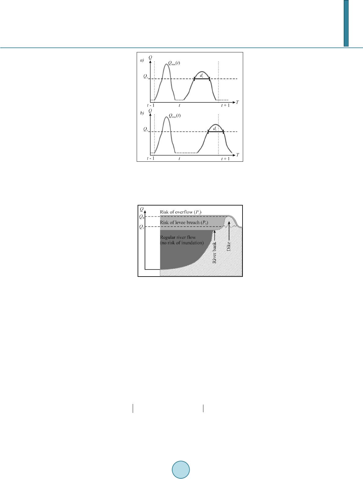

E. Bogdanowicz et al.
137
Figure 1. Definition of the threshold flow
discharge and duration in DqF model: a) the
flood wave of dt duration entirely in the year t;
b) the flood wave starts in the year t and conti-
nues in t + 1.
Figure 2. Two reasons of inundation—an illus-
tration.
The annual probability of inundation for embanked river reach is expressed as the total of probability of the
two exclusive events (Fl stands for “flood”) (see Figu re 2):
( )( )()
12
= +P FlPFlPFl
(1)
where the first term comes from the conventional FFA
( ) ( )
1 max
= >
B
PFlp QQ
(2)
The second term of Equation (1) defines the probability of inundation caused by levees breaching which
depends on both the flood persistency and levees resistance to high water stages which in turns depends on their
design and technical condition. Therefore the P2(Fl) is expressed as the integral of the product of the value of
the hazard index p(Fl|d) which is defined as the probability of levee breaching caused by the d-days duration of
flow over the flow level QA and of the pdf of the d—duration, i.e. f(d) for annual peak flows in the interval QA <
Qmax(t) < QB .
( ) ( )
( )
( ) ( )
2 max
0
d
+
∞
= <≤=⋅⋅
∫
AB
PFlpFlQQQhFl dfdd
(3)
where
f(d)—pdf of the duration d of flows above the alarm stage;
h(Fl|d)—the hazard index being the probability of levee breaching caused by a high water of the duration d.

E. Bogdanowicz et al.
138
The value of the hazard index h(Fl|d) tends to 0 for d going to 0 and to 1 for d going to infinity. The hazard
index h(Fl|d) is determined administratively for the river reach by the Regional Water Management Board based
on the technical assessment of flood embankments.
Note that collating the annual maximum high flow duration data for analysis one puts dt = 0 both for Qmax <
QA and Qmax > QB, i.e. the only one inundation yearly is considered and that caused by spilling over crest has the
priority over one caused by prolonged high stages. Furthermore note that the weaker is the relationship between
annual maximal values of peak flow and duration of flows above the alarm flow (QA) the more justified is the
separate analysis of the both random variables.
The ratio of probabilities P2 to P1 and their total is helpful to determine the actions to reduce the risk of
flooding, namely the strengthening or heighten the levees (or building parallel levees).
3. Formal Aspects of the Duration-Flow-Frequency Modelling
To address the flood risks arising from softening and washing out the river embankments, Bogdanowicz et al.
(2011) proposed to take as the subject of analysis the frequency of annual maximum uninterrupted duration, D
(in days), of flows over the flood alarm stage (QA), i.e. the duration (D) is considered as a random variable while
the alarm flow discharge (QA) is the fixed value (Figure 2).
The time-series of annual maximum uninterrupted duration, D (in days), of flows over the flood alarm flow
QA i.e. d = (d1, d2,…, dt,…, dT) is the subject of statistical modelling in stationary and non-stationary conditions.
The dt = 0, denotes that the QA has not been exceeded during the t-th year (Qmax(t) < QA) or that the peak flow
has exceeded the overtopping flow (Qmax(t) ≥ QB), which means that the priority of overtopping over breaching
is given and we rule out the possibility of two inundation floods of the two different origins within one year.
Note that the condition Qmax(t) ≥ QB is equivalent to the unconditional inundation, i.e. from Equation (2)
P1(Fl|Qmax(t) ≥ QB) = 1, while QB > Q(t) ≥ QA points only possible inundation (see Equation (3)).
Frequency analyses of hydrological sample with zero events have received relatively little attention. Still there
are several approaches for analysis of censored data, including probability plot regression, weighted-moment
estimators, maximum likelihood estimators, and conditional probability analyses (Gilliom & Helsel, 1986; Hass
& Scheff, 1990; Harlow, 1989; Helsel, 1990). A consistent approach to the frequency analysis of such data
requires using discontinuous probability distribution functions. Jennings and Benson (1969), Interagency
Advisory Committee on Water Data (1982), Woo and Wu (1989), Wang and Singh (1995) among others
developed empirical three-parameter models for frequency analysis of hydrologic data containing zero values.
When the available water stage records have been sampled in daily intervals, the
d
values are integer
numbers and in reality correspond to the duration (d – 0.5, d + 0.5), while in particular for d = 0 to the interval (0,
d + 0.5). If a flood starts at the end of a year and is continuing to the next year, the
d
value is derived for
whole flood and ascribed to the year t when culmination occurred. To get an insight into flood persistence
properties, the several threshold stages (QT) are considered but not only the alarm stage QA.
As far as the probability theory is concerned, the occurrence of zero events can be expressed by placing a
non-zero probability mass on a zero value, i.e. P(D = 0) ≠ 0, where D is the random variable, and Pis the
probability mass (e.g. Strupczewski et al., 2002, 2003; Weglarczyk et al., 2005). Therefore, the parent distri-
bution functions of such hydrologic series would be discontinuous (with discontinuity at zero) and, using the
theorem of total probability, their forms can be written as:
( )( )()()( )
1 ;1 βδ β = +−⋅gfddf dd

(4)
where β denotes the probability of the zero event, i.e., β = P(D = 0), f(d; g) is the conditional probability density
function (CPDF), i.e. f(d; g) ≡ f(d|D > 0), which is continuous in the range (0, +∞) with a lower bound of zero,
and g is the vector of parameters (containing β or not), δ(d) is the Dirac’s delta function and 1(d) is the unit step
function. Assuming the infinite upper bound for D seems acceptable and facilitates modelling. Due to
discretisied duration d intervals, the probability of exceeding the QA flow during one day only equals to
( )( )
12
12
d
+
−
= ⋅
∫
d
d
Pdfdd
. (5)
Hydrological samples with zero values are most frequently of exponential-like shape. Weglarczyk et al. (2005)
model the continuous part of (4) by two-parameter distributions, namely by Generalized Pareto, Weibull and

E. Bogdanowicz et al.
139
Gamma, estimating parameters by the maximum likelihood (ML) and the moments (MOM) methods.
4. Estimation of the Weight Parameter β
1) From the pdf of the duration d [Equation (4)] and the records d = (d1, d2,…, dt,…, dT) for given alarm flow
QA
From Equation (4) one can write the likelihood function as:
( )
( )
2
2
1
1
1; ββ
=
= ⋅−∏g
n
n
nj
j
L fd

(6)
where n1 and n2 denote the number of zeros and non-zeros values, respectively.
If β ∉ g, from ML-equations:
()
12
ln 0
1 ββ β
∂=−=
∂−
nn L
(7)
one can easily find that the ML-estimate of β is
1
12
ˆ
β =+
n
nn
(8)
i.e. β and g are estimated by MLM independently.
2) From CDF of annual maximum floods obtained from FFA
The better estimate of the β parameter in the sense of definition (Equation (9)), not its standard error, can be
obtained from the CDF of annual peaks providing the selected for Annual Maxima (AM) model fits well upper
tail data. Note that the D = 0, denotes that the QA has not been exceeded during the t-th year (Qmax(t)
≤
QA) or
that the peak flow has exceeded the overtopping flow (Qmax(t) > QB) where Qmax denotes the annual maximum
discharge, therefore, probability of zero value of D
( ) () ()
max max
ˆ ˆ ˆˆ
0 β ==<+ >=
AB
PDPQQ PQQ
(9)
Should be estimated from CDF of annual peak flows got from FFA rather than from the (0, 1) time series of
the d record. Having derived from FFA the CDF of the annual peaks
( )
( )
max
ˆˆ
, φ ≡h
max
GQ Q
where
ˆ
h
is the
vector of parameter estimates, one gets the estimate of β as
() ()
( ) max
ˆ ˆˆ
1 β == +−=
max AB
GQ QGQQ
(9a)
Note that if more than one flood appears in a year it may happen that the dt and the annual peak flow Qmax((t)
correspond to different floods.
Floods in excess ofQB are unique in Polish rivers, but if they were they should be in the FFA treated as of
unknown magnitude over the threshold QB, thus one deals with first order right censored sample.
5. Estimation of Parameters of the Continuous Part of Equation (4)
ML estimate of the parameters (g) of the continuous part of PDF (Equation 6), i.e. the conditional probability
density function (CPDF). f (d; g) ≡ f(d|D > 0) of f(d; g), can be obtained by solving the ML system of equations:
( )
2
1
ln ln;0 for
β
=
∂∂
== ∉
∂∂
∑
gg
gg
n
j
j
Lfd

(10)
Since the samples with zero values are most frequently of exponential-like shape, the following distribution
functions are recommended as candidates for f(dj; g) model: Exponential, Wei bull, Generalized Pareto,
Generalized Exponential and Gamma. Note that Exponential distribution is a special case of all other mentioned
above distributions. The detailed information on the models mentioned above with the methods of ML
estimation, one can easily find in hydrological and statistical literature, e.g. in Rao (2000) and for GE in Gupta
and Kundu (2000). Had the duration and peak flow were strongly linearly related to a legitimate adoption of a
common distribution function truncated the d distribution function to the positive half i.e. to d > 0.

E. Bogdanowicz et al.
140
The basic assumption in the classical Flood Frequency Analysis and the Duration-Flood-Frequency modelling
is that neither the adopted distribution function nor its parameters change in time it is possible to extend the
described methodology of the inundation risk assessment for the case of non-stationarity of flood regime.
6. Case Study—Szczucin at Vistula River (Southern Poland)
To illustrate how the proposed approach works in practice the Szczucin gauge (southern Poland) at the Vistula
River has been selected as the case study. The daily flows record covering the period 1951-2006 (n = 56 years)
was used in this study. At first the daily records have been controlled and tested with regard to the sharp
discontinuities and jumps in data—no particular irregularities have been detected (Figure 3).
The overtopping flow QB was assessed from the rating curve as 10,500 m3/s which roughly corresponds to
two-hundred-years return period of annual peak flow (Q0.5%), the base design value for the 1st class
embankments. In fact, there are no annual peak flows exceeding this value in the record. Therefore the QB value
does not affect the composition of the vector of observation values [dt]. The alarm threshold for the Szczucin
station QA = 1690 m3/s (which means flow of ca. 2-year return period, stage 660 cm), It gives n2 = 23 flood
hydrographs with Qmax above QA. The hazard index h(Fl|d) for QA = 1690 m3/s [Equation (3)] was assessed as:
( )
0.05for20 days
1for20 days
⋅≤ 
=>

dd
hFl dd
. (11)
i.e. the embankments can not withstand the pressure of high waters of more than 20 days.
A visual inspection of flood hydrographs reveals the variety of their shapes and, as a consequence, the d
distribution cannot be represented (or replaced rather) in FFA by Qmax distribution. It implies the analysis of both
d and Qmax by (perhaps) two different types of models. As a model for the parameters of the f function
Generalised Exponential (GE) distribution has been chosen (e.g. Gupta & Kundu, 2000):
()( )( )
1
; ,exp1exp
γ
γ
αγα α
α
−

= −−−

fdd d

(12)
where α > 0 is the scale parameter and β > 0 is the shape parameter.
Among the set of distributions mentioned in the previous section the GE distribution performs relatively well
in terms of the AIC value and shows stability of numerical ML solutions in estimation of f(d; g) parameters.
An additional argument for choosing the GE distribution is that being relatively recently derived was not to
our knowledge used in FFA.
However following on the model adopted for AM distribution which is Generalised Extreme Value (GEV)
distribution, the truncated at zero GEV distribution may be selected as the model of
o
f
, in particular in case of
a strong correlation between d(t) and Qmax(t).
The annual maxima are believed to be adequately described by the heavy-tailed distributions (e.g.
Strupczewski et al., 2011), so to cater for the Flood Frequency Analysis (FFA) for extreme values (i.e. annual
maxima) the values [Equation (8)] and P1(Fl) [Equation (2)] by means of Qmax series were calculated with the
three-parameter GEV distribution:
( )()( )
1
;,,exp1
γ
γ
γ
αγε ε
α

 
=−− −=





GEV
GqqG q
(13)
From the AM sample covering the period 1951–2006 (n=56 years) we got the ML estimates of GEV
parameters equal: location
ˆ
ε ≡
= 1260.02 m3/s, scale
≡
ˆ
α
= 671.39 m3/s and shape
ˆ
γ ≡
= –0.33.
Substituting for q into Equation (13) the QA value and then putting the corresponding probabilities to Equation
(9a), one gets the estimates of the weighting parameter
ˆ0.577
β =
. From Equation (8) we get quite similar
result, i.e.
ˆ33 560.559
β = =
and the confidence interval for proportion β includes the value estimated from
AM distribution [Equation (9)]. ML parameter estimates of GE applied for
o
f
are
ˆ3.2348
α =
and
ˆ0.8357
γ =
.
7. Assessment of Probability of Levee Breach along Szczucin Reach.
Since the event of levee breach is conditioned by the peak flow being in the range of [QA, QB], Equation (3) can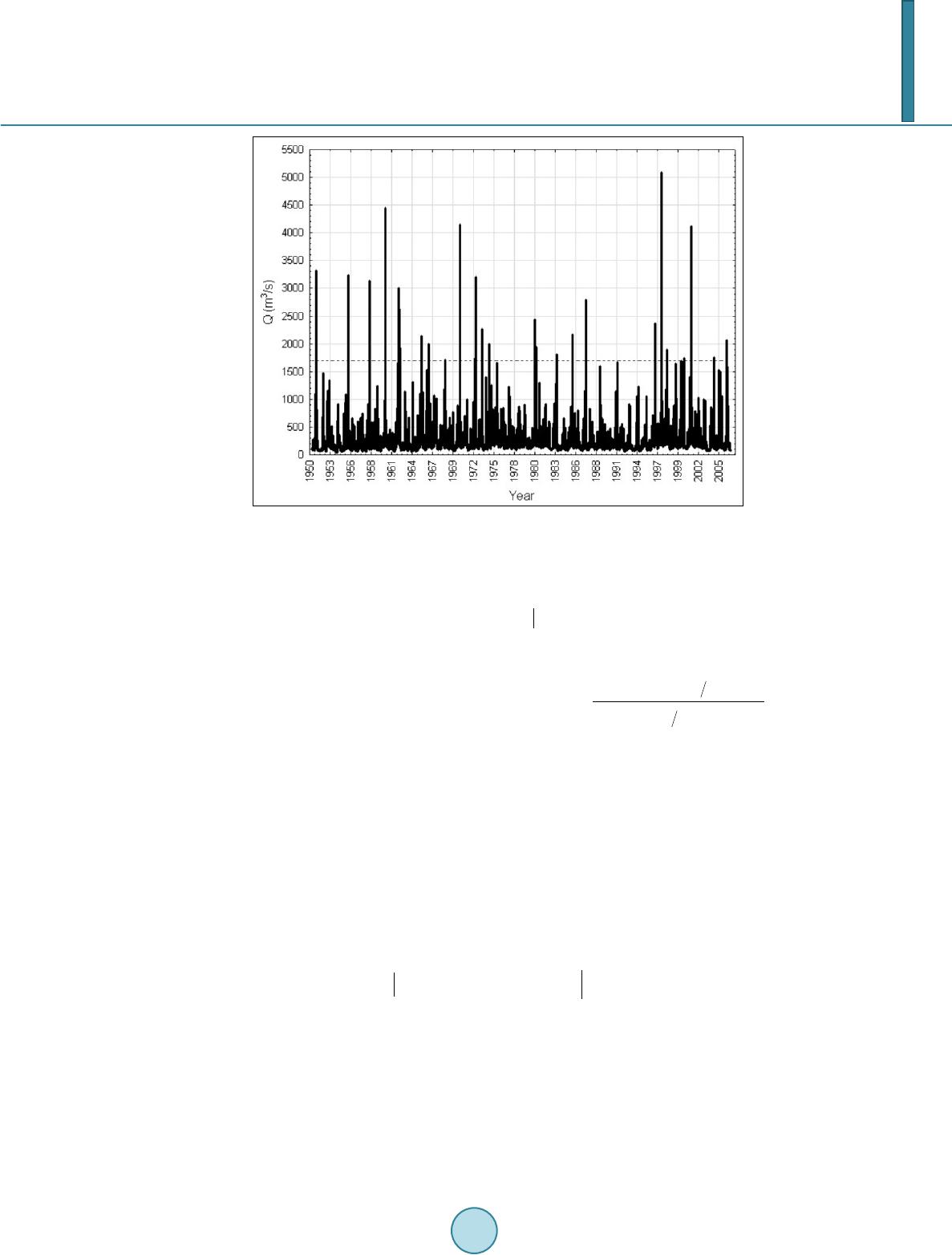

E. Bogdanowicz et al.
141
Figure 3. Hydrograph of the daily flows at the Szczucin gauging station. Hori-
zontal dashed line reflects the QA value.
be written as:
() () ()
( )
2
0
1d β
+
∞
= −⋅°⋅
∫
PFlpFl dfdd
(14)
The pdf for d > 0 takes the form
( )
() ( )
( )
0.1643
0.2441 exp3.4238
ˆ
1;3.4238,0.83570.423 1 exp3.4138 βα γ
⋅−
−⋅===
−−

d
fd d

(15)
while the ML estimate of
β was taken from Equation (9a) and it equals 0.577. Substituting it and the hazard
index function defined by Equation (11) into Equation (3a) and integrating one gets the annual probability of
levee breaching P2(Fl) = 0.064. Note that at the same time, and when the same GEV distribution is used the
probability of flood caused by exceeding embankment crest by annual peak flow, i.e. P1(Fl) = P(Qma x > QB =
10,500 m3/s) = 1 – G(QB) is equal to 0.005, i.e. it is almost insignificant (more than ten times smaller than P1),
hence, the overall probability of flood along Szczucin reach P = P1 + P2 = 0.069.
Variety of shapes of flood hydrographs can be evaluated by a measure of correlation strength between Qmax(t)
and d(t). Due to shape similarity of flood peak parts, a strong dependence between the peak flows (Qmax) and the
duration above the alarm flow (d) can take place. If it is a case, the probability P2(Fl) can be assessed on the
base of Qmax distribution g(Qmax). Assuming that d = ψ(Qmax) one can expressed in Eq.(15) the d variable by the
Qmax getting
( ) ( )
( )
( )
()
()
2maxmaxmax max
d ψ =<≤=⋅ ⋅
∫
B
A
Q
AB
Q
PFlpFlQQQh FlQgQQ
(16)
where per analogy to Euation (11) h(Fl|ψ(Qmax)) equals 0 and 1 for QA and QB, respectively. The Pearson’s
correlation coefficient r(Qmax, d) for Szczucin equals to 0.83.
Of course, when estimating the risk of a levee breach except the time of high water residence, more technical
parameters of levees should be analysed, such as the construction of the levee, the material used for its building,
its age, susceptibility to softening, the regime of the river, wind-induced waving and so on. All in all, those who
decided to build their houses in the river’s proximity behind the levees, sooner or later do experience a
catastrophe.

E. Bogdanowicz et al.
142
8. Conclusions
In the paper the new two-component model of flood waves, ‘duration of flooding-discharge-probability of
non-exceedance’ (DqF), with the methodology of its parameters estimation was proposed as a completion to the
classical FFA methods. Such model can estimate the duration (d) of stages (and flows) exceeding the assumed
magnitude with a certain probability which is of key importance when the river’s dikes are prone to the pro-
longed impact of high waters. The embankments may be weaken by the water, soak and eventually break—this
is the most frequent cause of floods in Poland. However, in this study the two main causes of inundation of em-
banked rivers, namely over-crest flow and wash out of the levees, were combined to assess the total risk of in-
undation. The proposed DqF modeling approach can be generalized to the non-stationary conditions. Therefore,
in addition to the maximum flow one should consider also the duration of high waters above the alarm flow QA
in a river channel. The model combined with the technical evaluation of probability of levees breach expressed
by the hazard index gives the annual probability of inundation caused by the embankment failure. The probabil-
ity of inundation is the total of probabilities of exceeding embankment crest by flood peak and the probability of
washout of levees.
The DqF modeling is the consequence of QdF approach developed by Javelle et al. (1999, 2000, 2002) and
Bogdanowicz et al.(2008) but in the first model the gravity is put on the probability of the certain duration above
alarming stage/discharge (QA) rather than on magnitude of flood itself (Qmax) like in the latter case.
The DqF model in the form of Equation (4) consists of two terms: β·δ (d) deals with the zero event, i.e. D = 0,
whereas the latter term (1 – β)·f(d;g)·1(d) stands for the events when the duration D > 0. In general both β and fº
in non-stationary case may depend on time. The maximum likelihood method (MLM) was proposed for estima-
tion of β and g parameters. In the non-stationary case it is convenient to describe the β (t; θ) by means of the lo-
gistic function (23). However, β and β (t; θ) can be also estimated by means of annual peak flows series, Qmax,
using the routine flood frequency techniques (FF) with distribution functions commonly used in FFA (e.g. GEV)
for stationary and non-stationary case, respectively. For f(dj; g) model the exponential-like shaped distribution
functions are recommended, such as: Exponential, Weibull, Pareto, Generalized Exponential, Gamma and simi-
lar.
The calculations for the Szczucin at the Vistula River case study have showed the similar results for the
weighting factor estimated by ML method from the duration time-series and from annual peaks time-series. The
peak flows that could overtop the embankments have not been detected in the Szczucin’s record (1951-2005).
According to the hazard function (11) the possibility of levees breaching increases almost tenfold the probability
of inundation.
Work on the application of the model DqF provides insight with respect to the shape of the flood hydrographs.
The shape of flood hydrograph varies according to a number of controlling factors in the drainage basin. For ex-
treme floods the decisive factor is the rainfall/snowmelt time distribution while the catchment variable charac-
teristics do not play a significant role. This results in shape similarity of peak parts of extreme flood waves of
the same origin. For smaller floods the observed shapes are more diversified. This often leads to the rather
strong, but not functional dependence between the main shape measures: duration d over a given threshold and
the peak flow Qmax. This correlation is stronger when one type of floods (rainfall or thaw origin) dominates at
the studied catchment closing profile. Then the questions arise if it is possible and profitable, in face of strong
enough dependence of the two variables, to replace d in the persistence analysis P2(Fl) by pdf of annual maxima
and if both variables have to be of the same probability distribution. Although substitution of d by Qmax seems to
be an effective way to simplify the calculations of the total risk of flooding, however this method reduce the ob-
served variability of d values and so distorts the description of flood dynamics. Due to not exact dependence or
not linear relation the distributions of d and Qmax can be different. It is difficult to point the lower limit of the co-
efficient of determination from which the above method could be used, but the weaker is the dependence, the
more justified is to analyze the both random variables D and Qmax separately.
The DqF model proved to be the important completion to the traditional FFA concentrating on maximal
seasonal or annual discharges. The DqF approach is especially useful in polish specific conditions where the
flood protection infrastructure is dated and often does not survive confrontation with prolonged pressure of high
waters.
Reliable data and information about floods are indispensable for better understanding the interactions between
rivers and flood protection system: embankments, reservoirs and polders. Improvement of statistical models is

E. Bogdanowicz et al.
143
essential for engineering design in general and in particular for implementation of flood risk mitigation
procedures. Not only has the DqF modelling shown that actual flood risk is greater than the risk assessed by
means of classical FFA but also provides quantitative measures which can be used in flood protection systems
planning, exploitation and conservation. This measure in form of dependence of inundation risk on river flow
(or water level) should be established for other hydrological stations on Polish rivers and their dimensionless
versions compared. The geographic information systems technique (GIS) could be used to indicate locations
prone to inundation, also the GIS can be a helpful tool to visualisation and testing trends in the structure of river
network and to the regional analysis. These results can constitute the theoretical background to a number of
practical decisions in water management issues.
Acknowledgements
This research project was partly financed by the grant of the Polish National Science Centre titled “Modern sta-
tistical models for analysis of flood frequency and features of flood waves”, decision nr DEC-2012/05/B/
ST10/00482 .
References
Bogdanowicz, E., Strupczewski, W. G., & Kochanek, K. (2011). Persistence as a Factor of Flood Hazard for Embanked Riv-
ers. EGU Leonardo Conference “Floods in 3D”, Bratislava, 23-25 November 2011, Abstract in Proceedings.
Gilliom, R. J., & Helsel, D. R. (1986). Estimation of Distributed Parameters for Censored Trace Level Water Quality Data-1.
Estimation techniques. Water Resources Research, 22, 1201-1206.
Gupta, R. D., & Kundu, D. (2000). Generalized Exponential Distribution: Different Method of Estimations. Journal of Sta-
tistical Computation and Simulation, 1-22.
Haas, C. N., & Scheff, P. A., (1990). Estimation of Averages in Truncated Samples. Environmental Science & Technology,
24, 912-919. http://dx.doi.org/10.1021/es00076a021
Harlow, D. G. (1989). Effect of Proof-Testing on the Weibull Distribution. Journal of Materials Science, 24, 1467-1473.
http://dx.doi.org/10.1007/BF02397087
Helsel, D. R. (1990). Less Than Obvious: Statistical Treatment of Data Below Detection Limit. Environmental Science &
Technology, 24, 1767-1774.
Interagency Advisory Committee on Water Data (1982). Guidelines for Determining Flood Flow Frequency. Bulletin 17B,
U.S. Department of the Interior, Geological Survey, Office of Water Data, Reston, Va.
Rao, A. R., & Hamed, K. H. (2000). Flood Frequency Analysis. CRC Press.
Strupczewski, W. G., Singh, V. P., & Weglarczyk, S. (2002). Physically Based Model of Discontinuous Distribution for Hy-
drological Samples with Zero Values. In S. Al-Rashe d, & A. A. Sherif (Eds.), Proceedings of the Int. Conf. On WaRMAR,
Kuwait. Surface Water Hydrology (pp. 523-537). Lisse: Balkema Publishers, Swets & Zeitlinger.
Strupczewski, W. G., Weglarczyk, S., & Singh, V. P. (2003). Impulse Response of the Kinematic Diffussion Model as a
Probability Distribution of Hydrologic Samples with Zero Values. Journal of Hydrology, 270, 328-351.
http://dx.doi.org/10.1016/S0022-1694(02)00309-8
Strupczewski, W. G., Kochanek, K., Markiewicz, I., Bogdanowicz, E., Weglarczyk, S., & Singh V. P. (2011). On the Tails
of Distributions of Annual Peak Flow. Hydrology Research, 42, 171-192. http://dx.doi.org/10.2166/nh.2011.062
Wang, S. X., & Singh, V. P. (1995). Frequency Estimation for Hydrological Samples with Zero Values. Journal of Water
Resources Planning and Management, ASCE, 121, 98-108. http://dx.doi.org/10.1061/(ASCE)0733-9496(1995)121:1(98)
Woo, M. K. & Wu, K. (1989). Fitting Annual Floods with Zero Flows. Canadian Water Resources Journal, 14, 10-16.
http://dx.doi.org/10.4296/cwrj1402010
Weglarczyk, S., Strupczewski, W. G., & Singh, V. P. (2005). Three-Parameter Discontinuous Distributions for Hydrological
Samples with Zero Values. Hydrologic Processes, 19, 2899-2914.