 Journal of Geoscience and Environment Protection, 2014, 2, 126-134 Published Online June 2014 in SciRes. http://www.scirp.org/journal/gep http://dx.doi.org/10.4236/gep.2014.23017 How to cite this paper: Zhu, Z. F. (2014). Minimum Wind Stress for the Occurrence of Blue Tide on the Southeast Shore of Tokyo Bay. Journal of Geoscience and Environment Protection, 2, 126-134. http://dx.doi.org/10.4236/gep.2014.23017 Minimum Wind Stress for the Occurrence of Blue Tide on the Southeast Shore of Tokyo Bay Zhong Fan Zhu College of Water Sciences, Beijing Normal University, Beijing, China Email: zhuzhongfan1985@gmail.com Received March 2014 Abstract In Tokyo Bay, blue tide is a phenomenon that seawater presents to be milky blue due to reflection of sunshine off surface water in which a large number of sulfur particles suspend. Its occurrence is because of coastal upwelling of the oxygen-depleted water at the bottom of the bay induced by the blowing of a northeasterly wind, consequently leading to many deaths of shellfish and some aquatic animals in the bay. In this study, an analytical solution of minimum wind stress for the oc- currence of blue tide on the southeast shore of the bay is presented based on a two-layered model, and comparison with observation data of blue tide from 2003 to 2010 shows the validity of this solution. The results of sensitivity analysis to all of parameters involved in this solution were also found to ag ree with qualitative understandings of blue tide phenomenon. Keywords Minimum Wind Stress, Blue Tide, Tokyo Bay 1. Introduction Tokyo Bay w as subject to the consequences caused by a rapid urbanization and an intensive industrial develop- ment. Large quantities of untreated domestic sewage and municipal sewage as well as industrial sewage, which contained large nitrogen and phosphorus loads, were discharged into Tokyo Bay, consequently influencing se- riously the development of the ecosystem in the bay. The input of these nutrient loads, with available sunlight in the surface and suitable temperature in spring or summer, promoted the excessive growth of phytoplankton. As a result, a phenomenon known as red tide (or algal bloom) took place, where the concentration of phytoplankton was so high that the color of seawater presented to be red. Red tide occurred frequently in Tokyo Bay, and its occurrence led to decreased biodiversity, toxin production and dissolved oxygen depletion in the bay. When phytoplankton died and fell into the bottom water due to gravity, some of them were largely decomposed by bacteria at the bottom. During this process, a large concentration of dissolved oxygen at the bottom was con- sumed, and consequently the bottom water became oxygen-depleted or even anoxic. On the other hand, fresh water discharge into the bay from several rivers and intermittent precipitation particularly from summer to au-  Z. F. Zhu tumn, along with seasonal temperature variation caused by surface heating and cooling, resulted in a well-mixed upper water with high temperature and low salinity and a lower water with low temperature and high salinity in the bay. As a result, a stable stratification developed, where the lighter upper water covered on the surface of the heavier lower water. This stable structure prevented a vertical circulation to bring dissolved oxygen from the surface to the bottom, thus enhancing the oxygen-depleted state of the lower water. Under anaerobic conditions, sulfate contained in the bottom water will be reduced into hydrogen sulfide. When a northeasterly wind as fre- quently observed blew on the surface, the well-mixed upper water will follow the wind in the downwind direc- tion, and the oxygen-depleted lower water will flow in the opposite direction to compensate, finally resulting in coastal upwelling of the bottom water from the bottom to the surface. During this process, a large amount of hy- drogen sulfide present in the lower water was oxidized to colloidal sulfur substances when they meet the oxygen in the atmosphere. When sunshine reflected off the surface water containing these sulfur substances, the color of seawater presented quickly to be blue–green, and this phenomenon has been termed as blue tide. Coastal up- welling of the oxygen-depleted bottom water accompanying the outbreak of blue tide phenomenon caused a large number of mortalities of fish and shellfish in the upper warm water, consequently resulting in a substantial economical loss to coastal fisheries in Tokyo Bay. Plenty of researches concerning blue tide have been carried out in the past from different perspectives (Go- myo et al., 1998; Ichioka et al., 2009; Kakino et al., 1987; Kataoka et al., 1989; Koibuchi & Isobe, 2007; Ma- tsuyama et al., 1990; Nakatsuji et al., 1991; Nakatsuji et al., 1995; Otsubo et al., 1991; Sasaki et al., 1993; Sa- saki et al., 1996). These research results are helpful to understand the mechanism of outbreak of blue tide phe- nomenon, and, based on them, this study presents the minimum wind stress for the occurrence of blue tide on the southeast shore of the bay by using an analytical solution in the context of a two-layered model. The layout of this paper is as follows. Section 2 introduces briefly the engineering background and derivation of the ana- lytical solution. Comparison with observation data from 2003 to 2010 is provided in section 3, and section 4 presents the sensitivity analysis of the solution to all of the chosen parameters. As a summary, section 5 shows the concluding remarks. 2. Engineering Background and Derivation of the Solution As shown in Figure 1, Tokyo Bay is located in the central part of main islands of Japan. Its main axis, mean width and average water depth are 50 km, 20 km and 15 m, respectively. When a northeasterly-oriented wind begins to blow on the surface of the bay, blue tide is frequently observed along the coastline from off Funabashi to off Ichihara. As described in Zhu and Isobe (2012), although the real coastline of the bay is complicated, we just consider the research domain to be a rectangular one with the length of 50 km, the width of 20 km and water depth of 15 m, respectively, as shown by real lines and one dashed red line just indicating the imaginary southwest shore in Figure 1. Figure 2(a) illustrates the dimensions of this domain ( is the width, and a right-handed Cartesian coordinate system is defined as follows: the origin is in the center of domain, the axis follows the northeast- erly wind, the axis is perpendicular to the length direction of the domain, and the axis is positive upward above the still surface level.). Considering that a northeasterly wind is imposed suddenly and uniformly over the surface of the whole water body, Zhu and Isobe (2012) analyzed the occurrence process of blue tide using a two-layered model which is consisted of the upper, well-mixed layer and the lower anoxic layer, separated by a density interface. Since the wind begins to blow on the surface, within a short time, the initial oscillation arising from the Coriolis force due to the rotation of the Earth does not influence the water body, so that a wind-driven current in the water body can be simply viewed as being in longitudinal section. The wind generates some surface waves and then these surface waves are reflected by two boundaries of the bay, which forms a standing wave group. Motion of this standing wave group causes the surface tilt with the southwest boundary up and the northeast shore down, further causing the surface to oscillate about an equilibrium tilt. Such an equilibrium tilt will be reached when all wave energy is completely dissipated and, at this point, barotropic pressure on the whole water body caused by this equilibrium tilt is in balance with surface wind stress. The imposed wind stress also causes the vertical mo- tions of the water body. Specifically, since the onset of wind stress, the thin layer water beneath the surface will follow instantly the wind downwind and, as the compensation, the rest layer water between it and density inter- face will flow upwind, as also schematically shown in Figure 2(b). This opposite motion makes the interface up 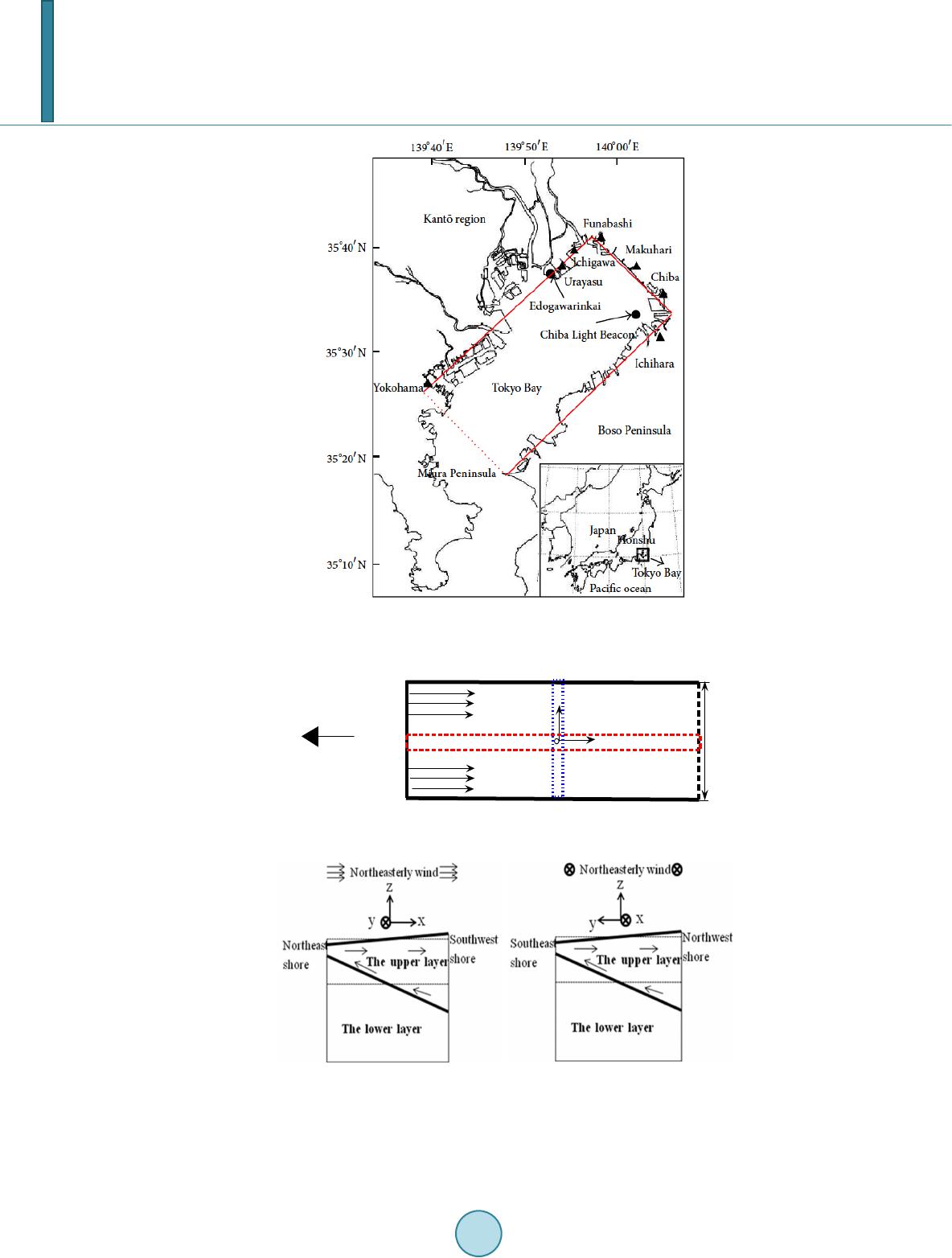 Z. F. Zhu Figure 1. Map of Tokyo Bay and the chosen research domain for the study of blue tide (Zhu & Yu, 2014). (a) (b) Figure 2. Dimensions of the chosen research domain (a) and schematic diagrams of coastal upwelling (b) and (c), caused by the continual blowing of a northeasterly wind. (b) (The wind direction is from the left to the right); (c) (The wind direction is perpendicular to the surface of this paper and inward). Northeasterly wind Northeast Northeast boundary Southeast boundary Northwest boundary Southwest boundary x y zb 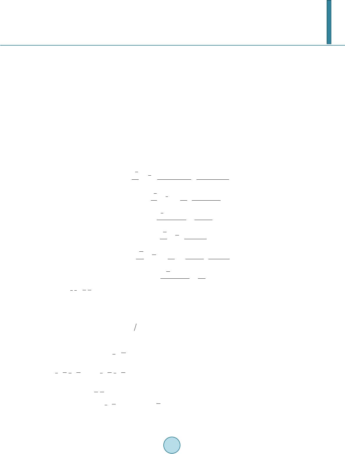 Z. F. Zhu at the northeast shore and down at the southwest shore of the bay, which is opposite to that of the surface. Simi- larly, this interface tilt is created by the motion of another standing wave group formed by some internal waves, thus also oscillating around an equilibrium position at which buoyancy force balances barotropic pressure caus- ed by the surface set-up. If wind condition is enough, the interface will intersect the surface at the northeast shore of the bay, and the lower anoxic water begins to touch and interact with dissolved oxygen at the surface, at this point, blue tide takes place. When the northeasterly wind continuously blows on the surface, the effect of the Earth’s rotation must be taken into account, and thus velocity direction of the upper layer water in the research domain is gradually deflected to the right of wind direction. In this case, the thin layer water beneath the surface will flow towards the northwest shore of the bay while the rest layer water between it and the density interface will flow in an opposite direction towards the southeast shore. Similarly, this opposite motion causes the corre- sponding tilt of the interface. If wind conditions are satisfied, the interface will also reach the surface and hence blue tide will occur on the southeast shore of the bay. Occurrence of blue tide on the southeast shore is just discussed in this study. In order to simplify the theoreti- cal method for calculating this case, all of parameters are simply assumed to be uniform along the axis (Zhu & Isobe, 2012), and we simply analyze the vertical motion in the transverse section of the bay as shown in Figure 2(c). Governing equations for the upper layer water and the lower one can be expressed as follows: () () '' 0 , sx Ix uf thh ττ υρζζ ρζζ ∂−= − ∂+− +− (1) ( ) ' , Iy fu g ty h τ υζ ρ ζζ ∂∂ +=− − ∂∂ +− (2) ( ) [ ] ( ) ; '' ty h ∂ −∂ −= ∂ −+∂ ζζζζυ (3) ( ) '' '' ' , Ix Bx uf th ττ υρζ − ∂−= ∂+ (4) () ( ) , ''' ' ' ' ζρ ττ ζζ ε ζυ + − + ∂ −∂ − ∂ ∂ −=+ ∂ ∂ h y g y guf t ByIy (5) ( ) '' '' h yt υζ ζ ∂+ ∂ = − ∂∂ (6) Where are vertically-averaged horizontal velocity components in directions of the upper and the lower layers, respectively, are thicknesses of the upper layer and the lowe-r one, respectively, are densities of the upper layer and the lower one, respectively, is the reference of wa-ter, are surface dis- placement and interfacial displacements, respectively, and are gravitational accele-ration and density con- trast between two layers ( ), is surface wind stress, are components of inter- facial and bottom shear stresses in directions, respectively, is the Coriolis coefficient, and is the time. Considering a specific steady state at which the surface and the interface just intersects on the southeast shor e when the northeasterly wind lasts for a infinitely long time, there should be a vertical circulation in each layer as shown by Figure 2(c), so . If the interfacial shear stress is simply assumed to be expressed in terms of the velocity difference between the upper layer and the lower one as, , () () ''' '' ,, I uu Cuu υυ ρυυ ∗−−= −− , wh ere are coefficients of interfacial shear stress of the upper layer and the lower one, respectively, similarly, bottom shear stress being expressed in terms of velocity of the lower layer as , where is the coefficient of bottom shear stress, it can be found readily that , and . At this point, for the upper layer, the force balance along 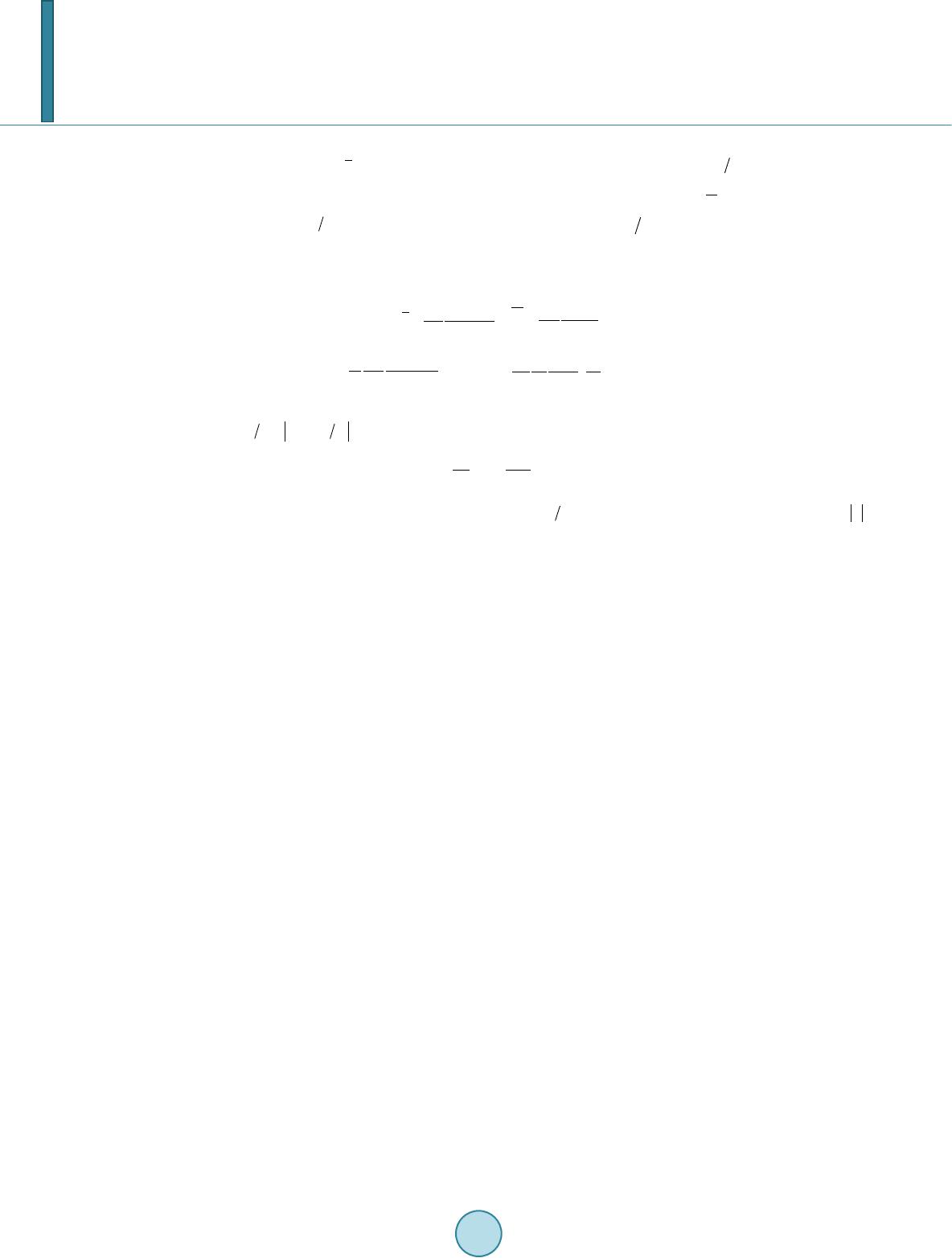 Z. F. Zhu direction is between wind stress and interfacial shear stress , an d the balance of forces along direction is among the Coriolis force , pressure gradient due to the surface displacement , as schematically shown by Figure 3(a); for the lower layer, interfacial shear stress simply balances bottom shear stress along direction, and the force balance along direction is among the Coriolis force , pressure gradient due to surface displacement and that due to interfacial displacement as also schematically shown in Figure 3(b). Substituting these expressions in Equation (1)-Equation (6) and considering all parameters at the steady state can yield , ; (7) ( ) y CC CC g f y BI IB sx ' 0 + −= ρ τ ζ , ( ) ( ) ' '' ' 0 1 sx BI I IB f yC CCy g CC τρ ζερ ρ = +− . (8) when the surface only intersect the surface on the southeast shore, the following mathematical relation should be satisfied: . Thus a wind stress can be gotten: ( 9) It can be found from Equation (8) that the large parameter results in the larger parameters and at the steady state, indicating that Equation (9) actually represents the minimum wind stress for the occurrence of blue tide on the southeast shore of the bay. 3. Comparison with Observation Data As presented in Zhu and Yu (2014), surface wind stress in Equation (9) is generally expressed to be a quadratic function of surface wind speed (Matsuyama et al., 1990; Wilson, 1960): , where is air density ( = 1.23 kg/m3), is surface drag coefficient (here = 1.30 10−3 is adopted, as presented in Mat- suyama et al. (1990) and Wilson (1960), and is the average wind speed measured 10 m above the still sur- face. Some typical parameter values in Equation (9) in case of Tokyo Bay are as follows: 20 km, 8.47 10−5∙s−1, 1000 kg/m3. Especially, a simple estimate regarding shows that it should be of the order of 10−4, so we simply chose the empirical value 10−4 in this preliminary study. Observation data sets of blue tide at the head of Tokyo Bay from 2003 to 2010 are available (Zhu and Isobe, 2012), and, among these data sets, those data sets of blue tide observed on the southeast shore of the bay are only chosen. Wind data set measured at Edogawarinkai shown in Figure 1(a) is simply adopted to represent wind condition across the whole bay (Zhu and Yu, 2014). By using this raw data set, the average speed of the northeasterly-oriented wind and the total duration are calculated. The starting point for calculating the wind duration across which the average wind speed is calculated corresponds to the first appearance of the northeas t- erly-oriented wind that can directly contribute to outbreak of blue tide, the ending point corresponds to the tim- ing at which blue tide just happens, as shown in Figure 4 as a typical example. As introduced in Zhu and Isobe (2012) in detail, for each real case of blue tide, value of minimum wind speed in Equation (9) should be different, because the density contrast and thickness of the well-mixed upper layer are closely related to stratification degree and they should differ one case by another case. In order to calcu- late them, a series of real-time measurement data from Chiba Light Beacon (CLB) also indicated in Figure 1(a) are used. Densities of the upper and lower layers can be calculated based on the temperature and salinity, and thickness of the well-mixed upper layer can be estimated from vertical distribution contours of temperature, sa- linity and dissolved oxygen. Here it needs to be mentioned that this study did not use spatially-averaged wind data and stratification data across the whole bay because of a lack of a long-term and real-time data measured at different locations of the bay beyond CLB. Table 1 summarizes the comparison result of the analytical solution with real cases from 2003 to 2010. The first big column shows date of the occurrence of blue tide on the southeast shore of Tokyo Bay from 2003 to 2010; the second column presents the calculated average wind speed along the north ea st-southwest direction and 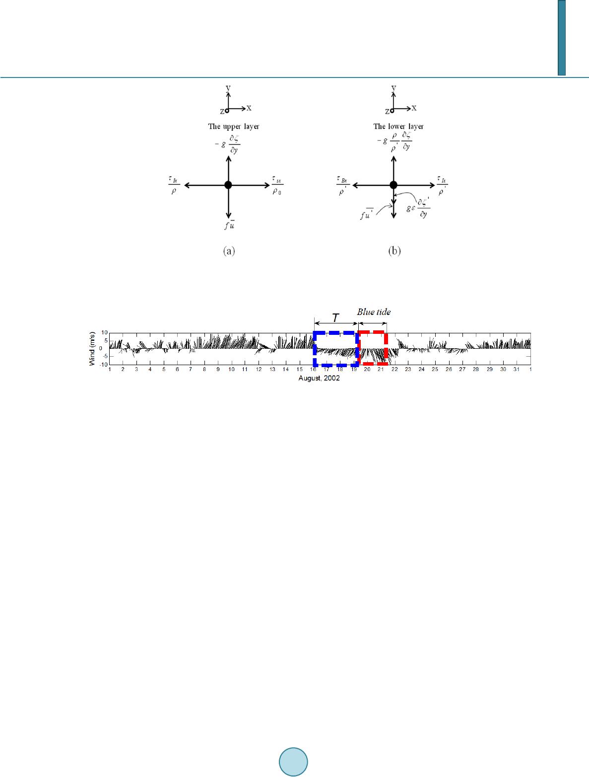 Z. F. Zhu Figure 3. Schematic diagram of the force balance for the upper layer (a), and that for the lower layer (b) when the two-layered fluid is in the steady state in the case of blue tide on the southeast shore of Tokyo Bay. Figure 4. Vector diagrams of surface wind measured at Edogawarinkai in Tokyo Bay in August, 2002. The orientation is as follows: the up points to the north, the down the south, the left the west and the right the east. The red dashed rectangle denotes the duration of an observed blue tide: the left dashed line shows the timing of the occurrence of blue tide, and the right shows the timing of its disappearance. The blue dashed rectangle denotes the duration of the northeasterly-oriented wind: the left dashed line shows the first timing of the occurrence of the northeasterly-oriented wind, and the right corres- ponds to the timing of the appearance of blue tide. wind duration; the third column shows the stratification degree for each case using measurement data sets from CLB (including densities of the upper and lower layers, thicknesses of the upper and lower layers). Using these values, the fourth column presents the calculated minimum wind speed fro m Equ ation (9). Whether the wind speed of each real case exceeds the calculated minimum wind speed is shown in the fifth column, which shows a good agreement between real cases and the solution. It can be concluded that the analytical solution shows a certain degree of validity. 4. Sensitivity Analysis Sensitivity of the analytical solution to all of parameters incorporated into it can be carried out by qualitatively analyzing Equation (9), and some results can be obtained as follows: 1) When density of the lower layer water with a fixed density for the upper layer water is increased, minimum wind stress will increase accordingly. This is because a heavy lower water layer has a large gravity against sur- face wind effect, thereby making coastal upwelling become difficult. This conclusion is consistent with the re- sults of numerical simulation of Matsuyama et al. (1990), which showed that coastal upwelling is prone to hap- pen in early autumn because during this period stratification becomes weak. This conclusion is also applicable to the case in which density of the upper layer water is decreased and density of the lower layer water is fixed. 2) When thickness of the upper layer water is increased, minimum wind stress needed for the occurrence of coastal upwelling will increase accordingly. This is because increasing thickn ess of the upper layer is equivalent to lengthening the spatial distance of coastal upwelling, thus making coastal upwelling get more difficult. 3) The wider the research domain is, the easier the occurrence of blue tide gets. This may be interpreted by virtue of geometry of the research domain: under the circumstance in which all of parameters keep the fixed  Z. F. Zhu Table 1. Comparison of the analytical solution with real cases of blue tide observed on the southeast shore of Tokyo Bay from 2003 to 2010 (based on measured data from Chiba Light Beacon). Blue tide on the southeast shore of Tokyo Bay wind Degree of stratification The analytical solution Equation (9) Does the average wind speed exceed the calculated minimum wind speed? Date of appearance speed/Wind duration (m/s)/(h) Surface temperature/ Surface salinity (˚C)/(psu) Bottom temp e r a ture/ Bottom salin (˚C)/(psu) Density of the upper layer (kg/m3) the lower layer (kg/m3) The initial thickness of the upper layer (m) The initial thickness of the lower layer (m) 2003 May 16- May 19 3.64/45 18/29.8 15.6/33 1021.48 1024.24 5.00 10.00 ≥ Yes Sep 22- Sep 24 5.52/47 22.8/31 20.4/33 1020.99 1023.27 5.00 10.00 ≥ m/s Yes 2004 Jul 28- Jul 31 6.06/48 26.4/29.8 20.4/33 1019.17 1023.27 5.00 10.00 ≥ m/s Yes 2005 May 31- Jun 1 5.10/61 18/30.6 16.2/33.40 1022.24 1024.55 5.00 10.00 ≥ m/s Yes Jun 15- Jun 17 4.57/68 19.2/32.2 16.8/33.60 1022.71 1024.47 5.00 10.00 m/s Yes Sep 6- Sep 7 4.27/37 25.2/27 21.6/33.0 1017.28 1022.73 2.50 12.50 ≥ m/s Yes Sep 26- Sep 30 4.24/138 21.6/31.8 20.4/33.0 1022.08 1023.27 3.00 12.00 ≥ m/s Yes Oct 12- Oct 17 3.89/72 21.6/31.8 21.6/33.20 1022.08 1022.88 5.00 10.00 ≥ m/s Yes 2006 Sep 13- Sep 18 4.15/69 24/31 22.8/32.80 1020.65 1022.29 4.00 11.00 ≥ m/s Yes 2007 Sep 2- Sep 4 4.08/84 25.8/29.4 21.6/33.00 1018.60 1022.73 4.50 10.50 ≥ m/s Yes Oct 16- Oct 18 4.06/48 21/31.8 21/33.00 1022.24 1023.00 4.00 11.00 ≥ m/s Yes 2008 Aug 22- Aug 28 5.40/40 26.4/29 21.6/32.60 1018.42 1022.42 4.00 11.00 ≥ m/s Yes Oct 9- Oct 10 3.33/55 22.2/31 21/33.00 1021.16 1023.00 3.00 12.00 ≥ m/s Yes 2009 May 29- May 31 2.85/39 18/31 16.8/33.00 1022.24 1024.01 4.00 11.00 ≥ m/s Yes Aug 31- Sept 1 4.84/46 24/29 21.6/32.20 1019.14 1022.12 5.00 10.00 ≥ m/s Yes 2010 Sep 9- Sep 10 3.87/43 27.6/27 25.2/32.20 1016.55 1021.26 5.00 10.00 ≥ m/s No Sep 15- Sep 21 3.68/44 26.4/29.8 22.8/33.00 1019.17 1022.45 3.00 12.00 ≥ m/s Yes Sep 24 4.36/48 24/31 22.8/33.20 1020.65 1022.60 5.00 10.00 Yes constants except the width of the domain, a wide bay should mean a larger displacement of the interface on the boundary of domain between the upper and lower layers, consequently making coastal upwelling become easier. 4) It is apparent that upwelling can happen more easily in the research domain with a high latitude (that is a large Coriolis coefficient). This is simply because a high latitude means the larger Coriolis force, which intensi- fies the vertical motion of the upper layer water and subsequently accelerates the interface tilt on the boundary of the domain. 5) It can be found that it is difficult for coastal upwelling to happen in the domain with a large coefficient of interfacial shear stress of the upper layer. This is because the two-layered fluid system with a large coefficient of  Z. F. Zhu interfacial shear stress corresponds to a large production of heat, further implying that a stronger wind is needed for the occurrence of coastal upwelling on the boundary of the domain. 5. Concluding Remarks In this study, an analytical solution of minimum wind stress for the occurrence of blue tide on the southeast shore of Tokyo Bay based on a two-layered model has been derived. Comparison with observation data of blue tide from 2003 to 2010 showed certain the validity of this analytical solution. The results of sensitivity analysis to all parameters involv ed in it were also found to agree with qualitative understandings of blue tide phenome- non. Acknowledgements This research is supported by National Key Technology Research and Development Program of the Ministry of Science and Technology of China (Number: 2013BAB05B04) and “the Fundamental Research Funds for the Central Universities” in China (Number: 2013NT50). References Csanady, G. T. (1973). Transverse Internal Seiches in Large Oblong Lakes and Marginal Seas. Journal of Physical Ocean- ography, 3, 439-447. http://dx.doi.org/10.1175/1520-0485(1973)003<0439:TISILO>2.0.CO;2 Gomyo, M., Sasaki, J., & Isobe, M. (1998). Field Observation of Aoshio at Dredged Areas in Tokyo Bay. Proceedings of Coastal Engineering, Japan Society of Civil Engineers, 45, 981-985 (in Japanese). Ichioka, S., Sasaki, J., Yoshimoto, Y., Shimosako, K., & Kimura, S. (2009). Analysis of Sulfide Dynamics Including Out- break of Blue Tide in Navigation Channels and Dredged Trench of Tokyo Bay. Proceedings of Civil Society B2 (Coastal Engineering), Japan Society of Civil Engineers, 65, 1041-1045 (in Japanese). http://dx.doi.org/10.2208/kaigan.65.1041 Kakino, J., Matsumura, S., Sato, Y., & Kase, N. (1987). Relationship between Aoshio, Blue-Green Turbid Water and Wind-Driven Current. Nippon Suisan Gakkuin, 53, 1475-1481 (in Japanese). http://dx.doi.org/10.2331/suisan.53.1475 Kataoka, S., Hirotaka, H., & Komatsu, A. (1989). On the Occurrence Condition of Blue Tide in the Inner Tokyo Bay. Pro- ceedings of Ocean Development, Japan Society of Civil Engineers, 5, 233-238 (in Japanese). Koibuchi, Y., & Isobe, M. (2007). Phytoplankton Bloom Mechanism in an Area Affected by E utrophication: Tokyo Bay in Spring 1999. Coastal Engineering Journal, 49, 461-479. http://dx.doi.org/10.1142/S0578563407001691 Matsuyama, M., Touma, K., & Ohwaki , A. (1990). Numerical Experiments of Upwelling in Tokyo Bay in Relation to “Aoshio” (The Upwelled Anoxic Blue-Green Turbid Water). Bulletin on Coastal Oceanography, 28, 63-74 (in Japanese). Nakatsuji, K., Nagasaka, S., & Muraoka, K. (1991). Basic Experiments on Upwelling of Anoxic Water “Aoshio ” Observed in Tokyo Bay, Japan. Proceedings of Hydraulic Engineering, Japan Society of Civil Engineers, 35, 603-608 (in Japanese). Nakatsuji, K., Yoon, J. S., Yuasa, T., & Muraoka, K. (1995). The Relationship between Wi nd-Driven Stratified Flow and Occurrence Mechanism of Blue Tide. Proceedings of Coastal Engineering, Japan Society of Civil Engineers, 42, 1066-1070 (in Japanese). Otsubo, K., Harashima, A., Miyazaki, T., Yasuoka, Y., & Muraoka, K. (1991). Field Survey and Hydraulic Study of Aoshio in Tokyo Bay. Marine Pollution Bulletin, 23, 51-55. http://dx.doi.org/10.1016/0025-326X(91)90649-D Rao, D. B. (1966). Fr ee Gravitation Oscillations in Rotating Rectangular Basins. Journal of Fluid Mechanics, 25, 523-556. http://dx.doi.org/10.1017/S0022112066000235 Sasaki, J., Isobe, M., Watanabe, A., & Gomyo, M. (1993). The Phenomenon Regarding the Anoxic Water and a Model of Seasonal Variations of Temperature and DO in Tokyo Bay. Proceedings of Coastal Engineering, Japan Society of Civil Engineers, 40, 1051-1055 (in Japanese). Sasaki, J., Isobe, M., Watanabe, A., & Gomyo, M. (1996). Study on Scale of Blue Tide in Tokyo Bay. Proceedings of Coastal Engineering, Japan Society of Civil Engineers, 43, 1111-1115 (in Japanese). Ueno, S., Nadaoka, K., Ishimura, A., & Katsui, H. (1992). Analysis on the Upwelling Due to Wind in Tokyo Bay Based on NOAA-AVHRR Data. Proceedings of Coastal Engineering, Japan Society of Civil Engineers, 39, 256-260 (in Japanese). Wilson, B. W. (1960). Note That Surface Wind Stress over Water at Low and High Wind Speeds. Journal of Geophysical Research, 65, 3377-3382. http://dx.doi.org/10.1029/JZ065i010p03377 Zhu, Z., & Isobe, M. (2012). Criteria for the Occurrence of Wind-Driven Coastal Upwelling Associated with “Aoshio” on the Southeast Shore of Tokyo Bay. Journal of Oceanography, 68, 561-574. http://dx.doi.org/10.1007/s10872-012-0119-7  Z. F. Zhu Zhu, Z., & Yu, J. (2014). Estimating the Occurrence of Wind-Driven Coastal Upwelling Associated with “Aoshio” on the Northeast Shore of Tokyo Bay, Japan: An Analytical Model. The Scientific World Journal, 2014, 1-11. http://dx.doi.org/10.1155/2014/769823
|