Journal of Power and Energy Engineering, 2014, 2, 10-21
Published Online June 2014 in SciRes. http://www.scirp.org/journal/jpee
http://dx.doi.org/10.4236/jpee.2014.26002
How to cite this paper: Sridech, W. and Ch itso m b oo n , T. (2014) The Design of Stall-Regulated Wind Turbine Blade for a
Maximum Annual Energy Output and Minimum Cost of Energy Based on a Specific Wind Statistic. Journal of Power and
Energy Engineering, 2, 10-21. http://dx.doi.org/10.4236/jpee.2014.26002
The Design of Stall-Regulated Wind Turbine
Blade for a Maximum Annual Energy Output
and Minimum Cost of Energy Based on a
Specific Wind Statistic
W. Sridech*, T. Chitsomboon
School of Mechanical Engineering, Institu te of Engineering, Suranaree University of Technolo gy,
Nakhonratchasima Province, Thailand
Email: *winona13_me@hotmail.com
Received April 2014
Abstract
The design of a stall-regulated wind turbine to achie ve a maximum annual energy output is still a
formidable tas k fo r engineers. The design c oul d be carrie d out us ing an average wind speed to-
gether with a stand ard statistical distribution such as a Weibull with k = 2.0. In this study a more
elaborated design will be attempted by also considering the statistical bias as a design crit eri on .
The wind d at a used in this study were collec ted from three areas of the Lamtakong weather sta-
tion in Nakhonratchasima Provice, the Khaokoh weather station in Phetchaboon and the Sir ind-
horn dam weather station in Ubonratchathani, Thailand. The objective is to de sig n a best aerody-
namic configurations for the blade (chord, twist and pitch) using the same airfoil as that of NREL
Phase VI win d turbine. Such design is carried out at a design wind speed p oi n t. Win d turbine
blades were optimized f or bo th maximum annual energy production and minimu m cost of energy
using a method that take into account aerodyn amic and structural considerations. The work will
be carried out by the program “SuWiTStatwhich was developed by the auth ors and based on BEM
Theory (B lade Element Momentum). Another side issue is the credibility of the We ibu ll statis ti c in
representing the real wind measur emen t. This study uses a regression analysis to determine this
issue.
Keywords
Component, Wind Turbine Blade Design, Annual Power Yi eld, Local Wi nd Statistic, Cost of Energy
1. Introduction
To optimize the performance of fixed speed or stall-regulated wind turbine is a complex procedure according to
the several trade-off decisions. This type of wind turbine is mostly a small and medium size that is suitable for a
*Corresponding author.
W. Sridech, T. Chitsomboon
11
household utilization in the remote areas. The initial capital cost of investment is likely low due to the unneces-
sary intelligent control system, therefore installing the stall-regulated wind turbine in the low wind sites could be
the attractive choice. Merely, by optimizing the aerodynamic efficiency of the rotor, the best wind turbine could
produce the maximum annual yield for a given Weibull wind speed distribution.
Another important factor of designing the optimal rotor for the specific wind sites is the qu ality of the meas-
ured wind speeds. There are several parameters which have an effect on the quality of the measured wind speeds
namely period of time for collecting wind data (weekly monthly or yearly), frequency of collecting data includ-
ing the accuracy of the instruments, and so on. An acceptable wind data should be collected at least within 2
years [1]. Its frequency depends on the capability of the instrument which was collecting the data every minute.
Afterwards the hourly mean wind speed was determined in order to reduce a large number of data and evaluate
the statistical parameters.
The objectives of the present study are to maximize the annual energy (AEP) and to minimize the co st of
energy (COE) produced by the optimal wind turbine. The iterative approach was utilized in order to complete
the blade shape optimization by the aerodynamic model based on BEM theor y.
According to this study fo cu ses on a small wind turbine, therefore the initial cost of wind turbine would be
evaluated from the cost of blade due to its weight.
2. Study of Wind Statistic
The measured wind speeds u sed in this study was acquired from 3 meteorological stations at Lamtakong in
Nakhonratchasima, Khaokoh in Phetchaboon and Sirindhorn dam in Ubonratchathani. Lamtakong is located
between 14˚47'58"N latitu de and 101˚33'32.2"E longitude whereas Khaokoh is located between 16˚37'56.69"N
latitude and 100˚59'51.70"E longitude and Sirindhorn dam is located between 15˚12'13.87"N latitude and
105˚25'28.86"E longitude. All data was collected from 2006 -2008 at the height of 661 m above sea level and has
been supported by the Electricity Generating Author ity of Thailand.
2.1. The Real Wind Distribution
The frequency distribution of the measured wind speeds is mostly presented as a wind speed histogram with a
bin width of 1 m/s [2]. It can be calculated from the Equation (1).
k
n
iiI
H
Iv
Wn
VA
vf
k
∈=
=
,
.
)(
)(
1
( 1)
where
n
is the number of hourly mean wind speed da ta of the sample,
W
is bin width and
)(uA k
I
is the
indicator function of the interval
k
I
, wh i ch is 1 provided that
k
Iu
and is otherwise 0. Each interval is equal
to 1 according to the bin width setting. Figure 1 shows the frequency of the individual wind speed calculated
from Equation (1).
2.2. Weibull Distribution
The measured frequency distribution is mostly fitted with the Weibull distribution function which is quite flexi-
ble due to its two parameters as shown in Equation (2 )
(2)
where
V
is instantaneous wind speed,
k
is shape parameter and
c
is scale parameter [m/s],
086.1
=V
k
V
σ
,
)/11( k
V
c
=
And
V
is mean wind speed can be calculated from following relatio n
W. Sridech, T. Chitsomboon
12
(a)
(b)
(c)
Figure 1. The measured wind speeds histogram. (a) at Lamtakong in Nakho-
nratchasima; (b) at Khaokoh in Phetchaboon; (c) at Sirindhorn dam in Ubo-
nratchathani
0246810 12 14 16 18 20
0
0. 02
0. 04
0. 06
0. 08
0. 1
0. 12
0.14 p
wind speed [m/s]
Probability Distribution
0 2 4 681012 1416
0
0.04
0.08
0.12
0.16
0.2
wind speed [m/s]
Probability Distribution
W. Sridech, T. Chitsomboon
13
)/11( kcV +Γ=
,
dt
te
x
xt
−−
0
1
)
(
The W eibu ll distribution curve and statistical parameters corresponding to the measured wind speeds are ex-
pressed in Figure 2 and Table 1, r espectively.
(a)
(b)
(c)
Figure 2. Weibull distribution curve. (a) at Lamtakong in Nak-
honratchasima; (b) at Khaokoh in Phetchaboon; (c) at Sirind-
horn dam in Ubonratchathani.
0246810 12 14 16 18 20
0
0. 02
0. 04
0. 06
0. 08
0. 1
0. 12
0. 14
wind speed [m/s]
Probability Distribution
1357911 13 15 17 19
0
0. 02
0. 04
0. 06
0. 08
0. 1
0. 12
0. 14
p
wind speed [m/s]
Probability Distribution
1357911 13 15 17 19
0
0. 02
0. 04
0. 06
0. 08
0. 1
0. 12
0. 14
p
wind speed [m/s]
Probability Distribution
W. Sridech, T. Chitsomboon
14
Table 1. The statistical parameters at the three case study site.
Nakhonratchasima Phetchaboon Ubonratchathani
c 7.2427 m/s 6.9867 m/s 4.0096 m/s
k 2.3173 2.2089 1.8358
Variance 8.6374 8.7513 4.0475
mean 6.4170 m/s 6.1877 m/s 3.5625 m/s
3
3
()V
9.4700 m/s 9.3500 m/s 5.9900 m/s
R2 0.9628 0.9511 0.8833
The
2
R
considering between Weibull distribution function and the frequency distribution of the measured
wind speeds can be calculated from Equation (3).
=
=
−=
N
ii
N
iii
p
p
p
p
R
1
2
1
2
2
)(
)
ˆ
(
1
(3)
where
i
p
is the relative fr eq uency of the sample given by Equation (1),
i
p
ˆ
is the probability obtained from
Weibull function at each interval
k
I
,
p
is the mean of the total
i
p
alues and
N
is the total number of
intervals.
In consequence,
2
R
corresponding to the three case study sites namely Nakhonratchasima, Phetchaboon and
Ubonratchathani are 0.9628, 0.9511 and 0.8833, respectively. According to
2
R
represents the credibility of
Weibull distribution fitted by Weibull function and measured wind speeds, whe n it reaches to unity that means
the Weibull distribution is good agreement with the frequency distribution of the measured wind speeds. There-
fore, the Weibull distr ibutions f ro m the case s tud ies were proper to p redict th e prob ability of the wind statistic in
those sites.
3. Aerodynamic Modeling
BEM Theory is the most widely used method of calculating the preliminary performance of wind turbine due to
its low computational demand and reasonable accuracy. This work will be carried out by the program “Su-
WiTStat” which based on BEM Theory in order to optimize a rotor performance by a given local wind statistic
[3]. In this study, the wind speeds which produced the maximum wind power density,
3
3()V
, were chosen to be
the design wind speeds as shown in Table 2.
The NREL Phase VI wind turbine with rated power of 19.8 kW was chosen to be the original model [4]. It has
two twisted blades, a variable chord along the blade, and a rotor diameter of 10.1 m. The aerodynamic cross-
section is the S809 airfoil and is constant along the blades. The pitch angle is three degrees and rotational veloc-
ity is 72 rev/min. Thereby the design parameters are chord, twist and pitch. The program was iteratively search-
ing the optimal design parameters which provided the maximum power coefficient of each element calculated
by Equation (4):
drrVdPCdrrP
ρπ
3
,/=
(4)
where
2
1(sincos )
2
rdL rDr
dPNV rCCCdr
ρ ϕϕ
= Ω−
(5 )
4. Optimization
The design of the individual stall-regulated wind turbine, two objective functions were considered: maximum
AEP and minimum COE. The AEP was calculated by Equation (6)
8760( )( )
t
v
AEPP VfVdV= ×
(6)
W. Sridech, T. Chitsomboon
15
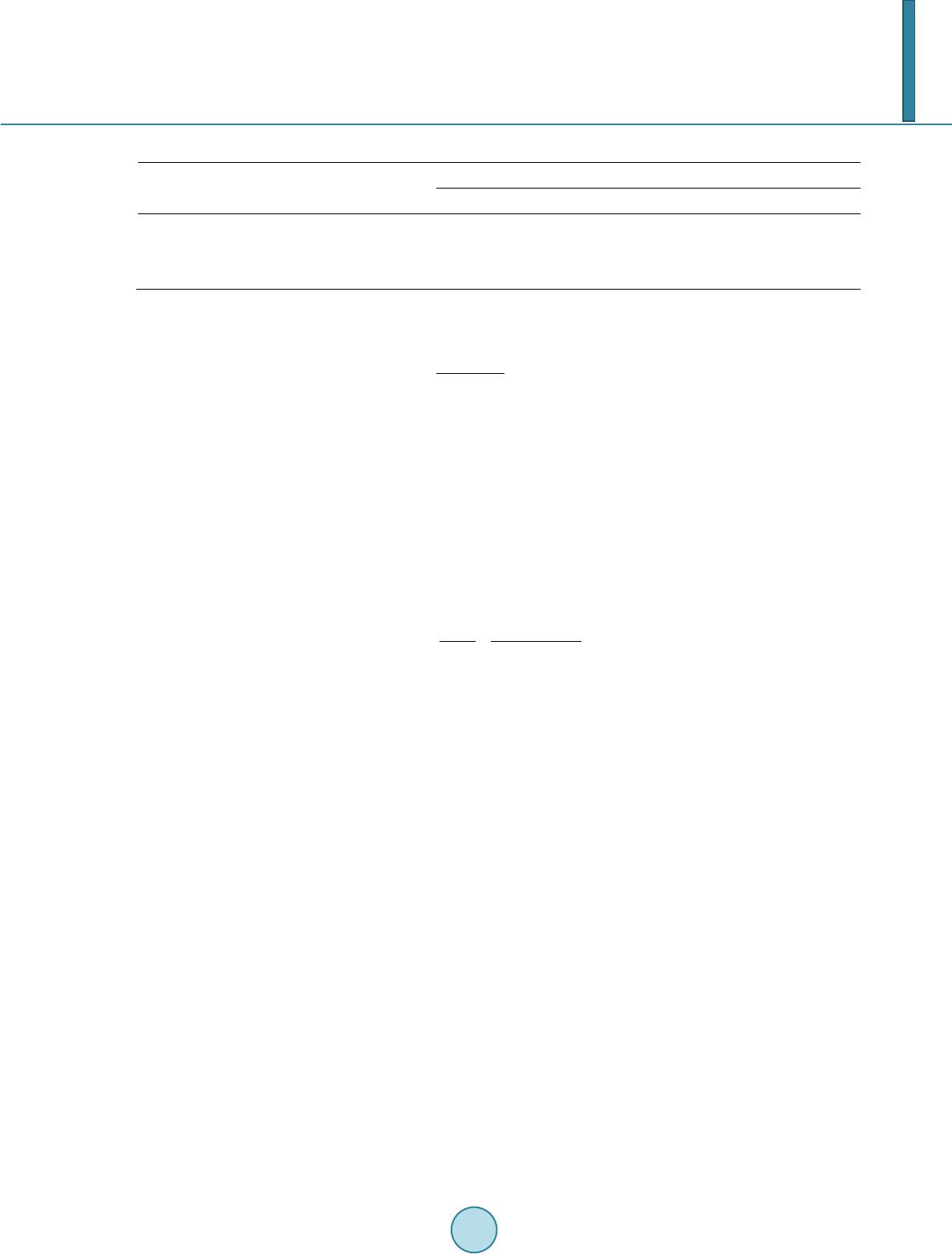
Table 2. AEP and COE of the optimized and the original wind turbine.
Area AEO [MW.h/year]
Original Smoothed
Nakhonratchasima 40.96 52.40
Phetchaboon 38.52 49.08
Ubonratchathani 12.51 14.06
where Pt was power of wind turbine produced at instantaneous wind speed.
The worthy of investment normally evaluated by COE which was calculated using the following equation [5]:
&
TC BOS
COEFCR OM
AEP
+
= ×+
(7)
In this equation, TC was the turbine cost ($/kW.h) [6]. For the balance of station BOS varied with the ma-
chine rating ($200/kW). The fixed charge rate FCR was 11%/year. The AEP was considering to be 98% availa-
bility. Finally, the operation and maintenance O&M was fixed at $0.01/kW.h.
From Equation (7), TC depends on blade cost which was determined according to its weight. Assuming the
blades were manufactured by E-glass using price of $20/kg where the blades represent 20% of the total turbine
cost.
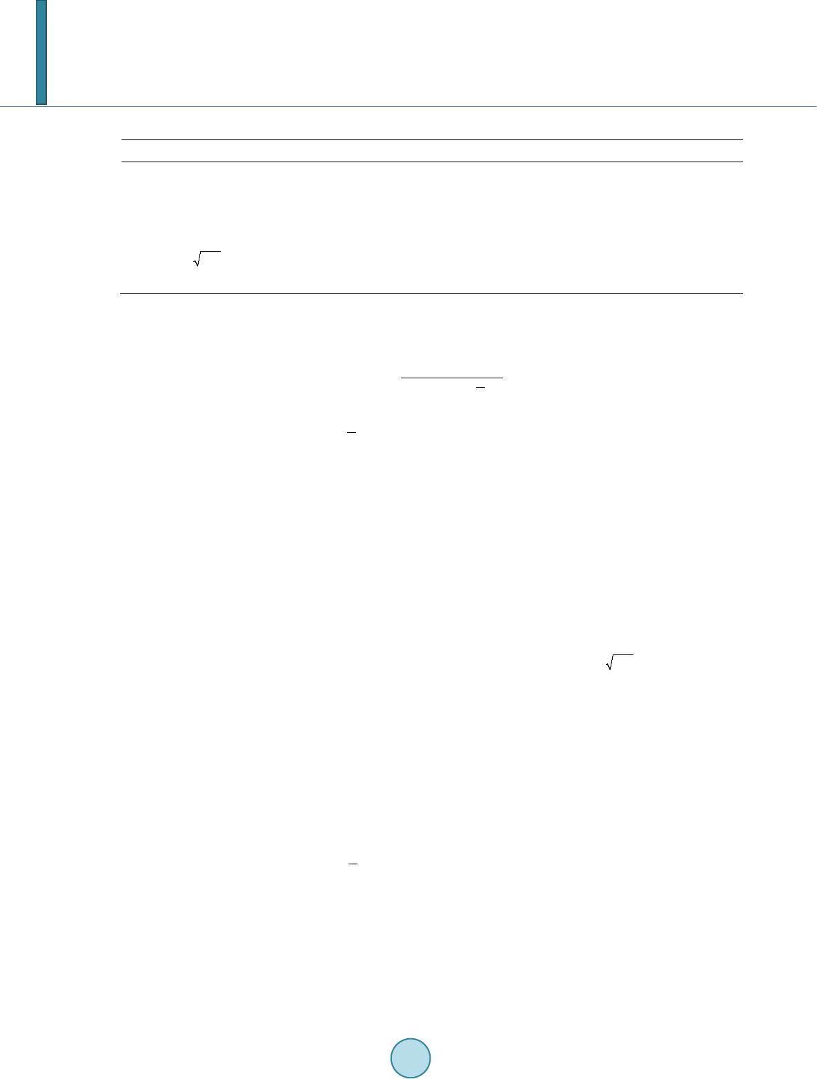
For evaluating the blades weight needed to know the skin thickness distribution along the blade. The skin thick-
ness was determined according to the maximum allowable stress (
max
σ
) corresponding to the material strength
of 110 MPa. If the residual stresses were taken into account, the
max
σ
equal to 94 MPa was used.
The total stress acting on blade composed of two components, first tensile stress due to centrifugal force and
stress due to bending moment, as shown in Equation (8):
[ ]
() ()/2
()
() () ()
r
Mr tr
Fr
rAr Ir
σ
= +
(8)
where
max ()r
σ χσ
=
and a Safety margin
χ
equal to 10. The cross-section was modeled as an I-beam with-
out a shear web as shown in Figure 3. It represented the overall skin thickness that was subjecting the load.
The maximum stress acting on blade was calculated in the condition that wind turbine was parked and fully
exposed to the storm. According to the International Electrotechnical Commission (IEC) [7], the IEC 50-year
extreme wind speed for a wind Class II (59.5 m/s) was used to compute the blade loads. In consequence, the
minimum skin thickness, blade weight and blade cost as well as turbine cost were determined.
5. Result and Discussion
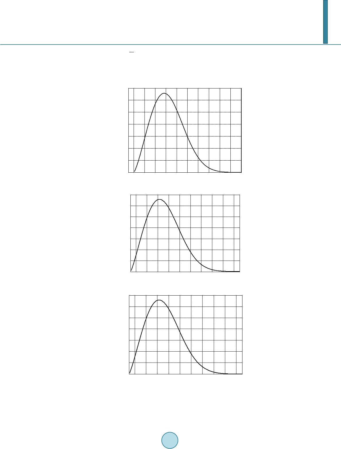
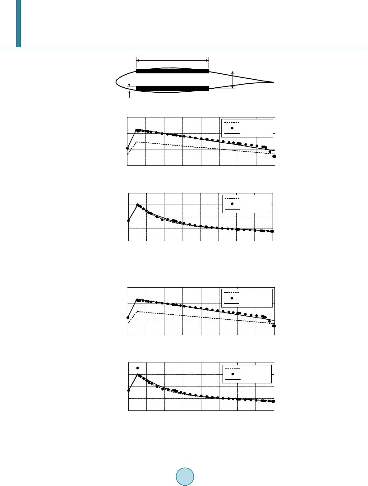
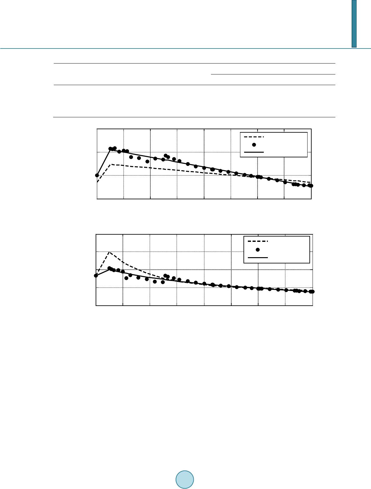
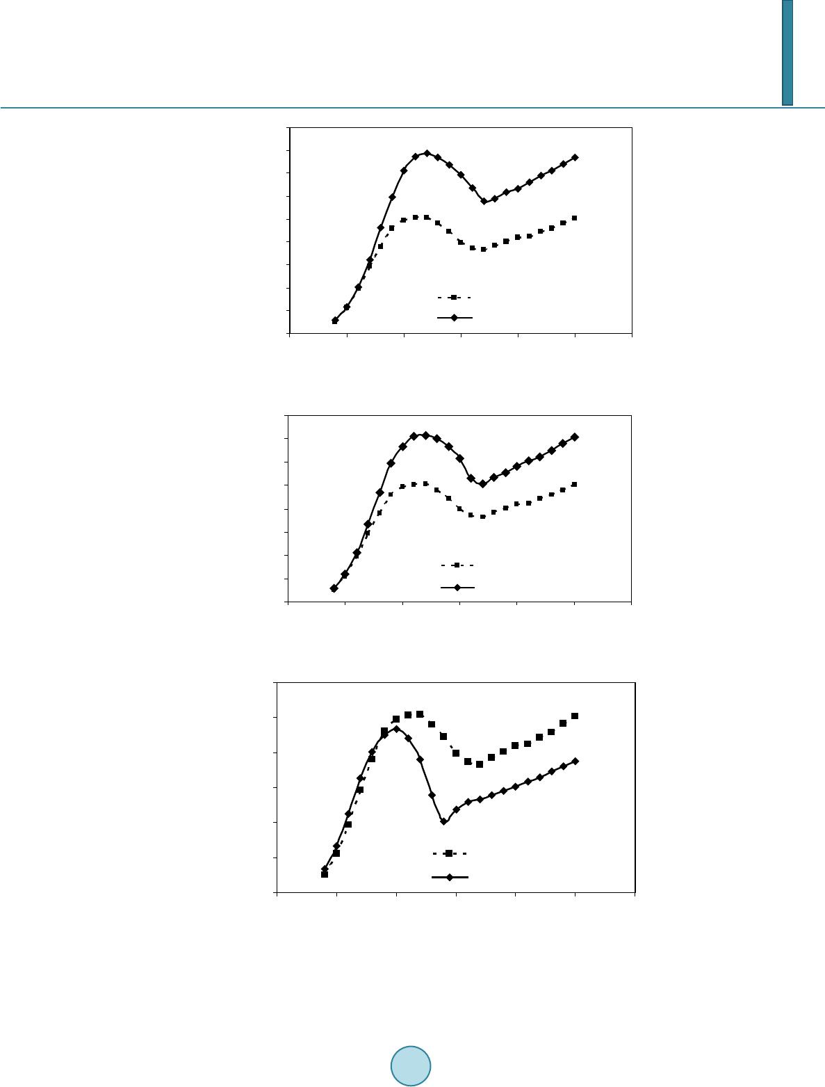
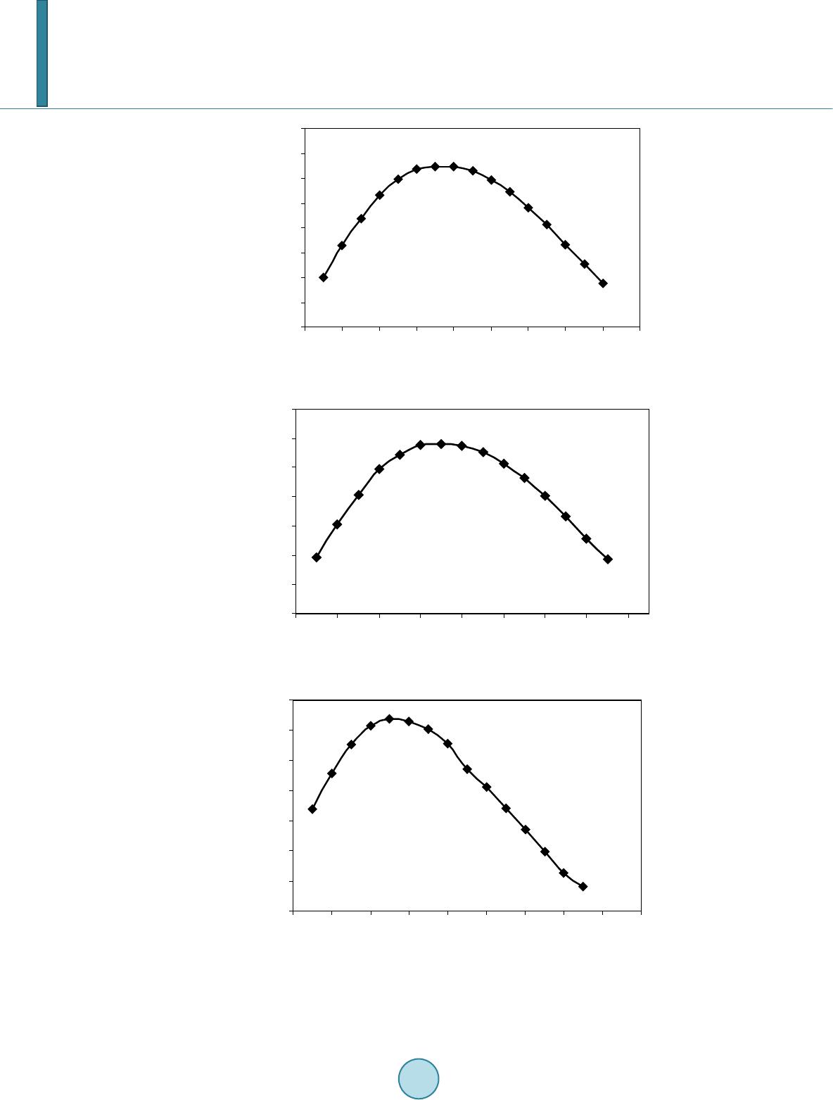
The op timal blade shapes for each case study are shown in Figures 4-6. In the optimization process, blade was
divided into many elements so that the number of elements then brought about the discontinuity of the op timized
points. However, increasing the number of elements made more reliable results but consumed more computa-
tional resource as well. Hence, the smoothed line was made for a feasib ility of blade manufacturing. In addition,
wind turbine with smoothed blades produced higher performances compared with the original one as shown in
Figure 7 and Figure 8, particularly oper ating at the mean wind speeds of the studied sites.
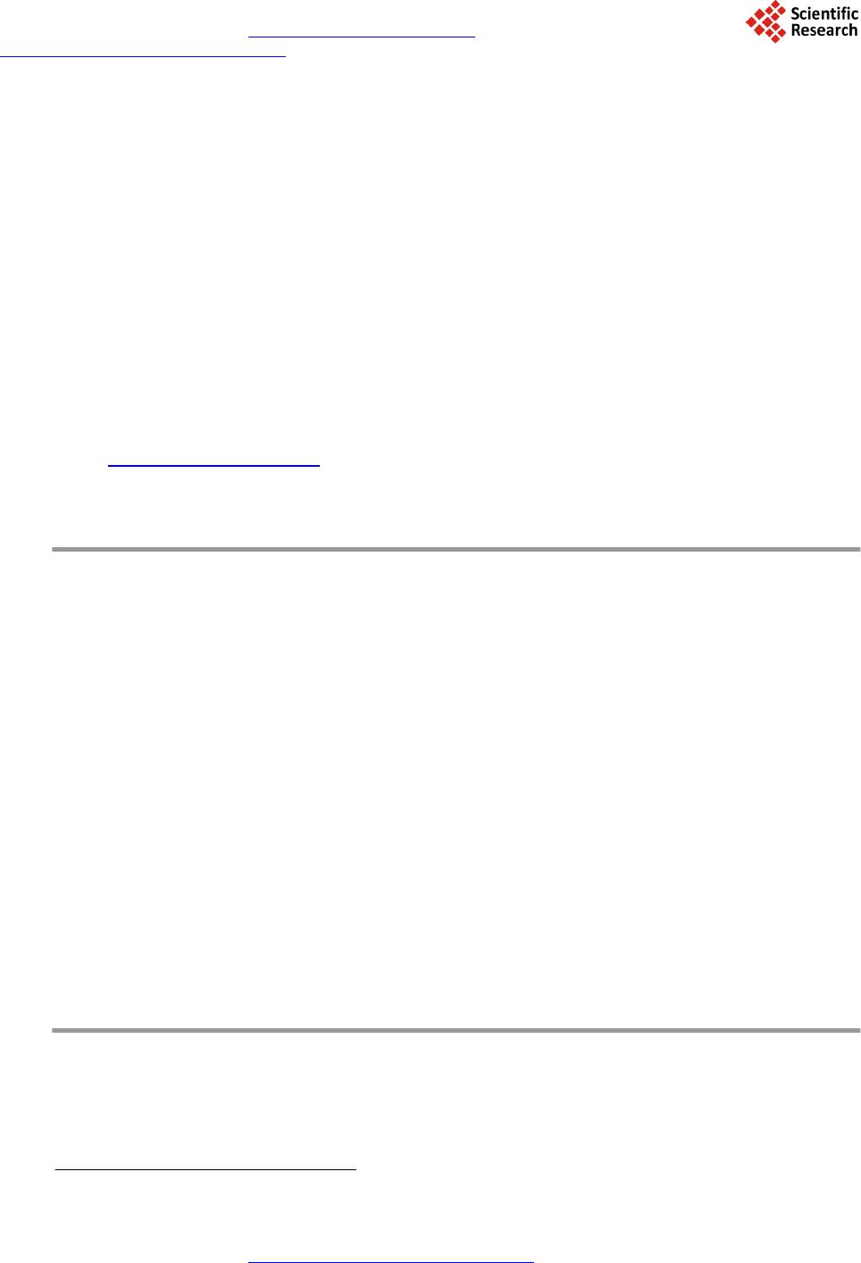
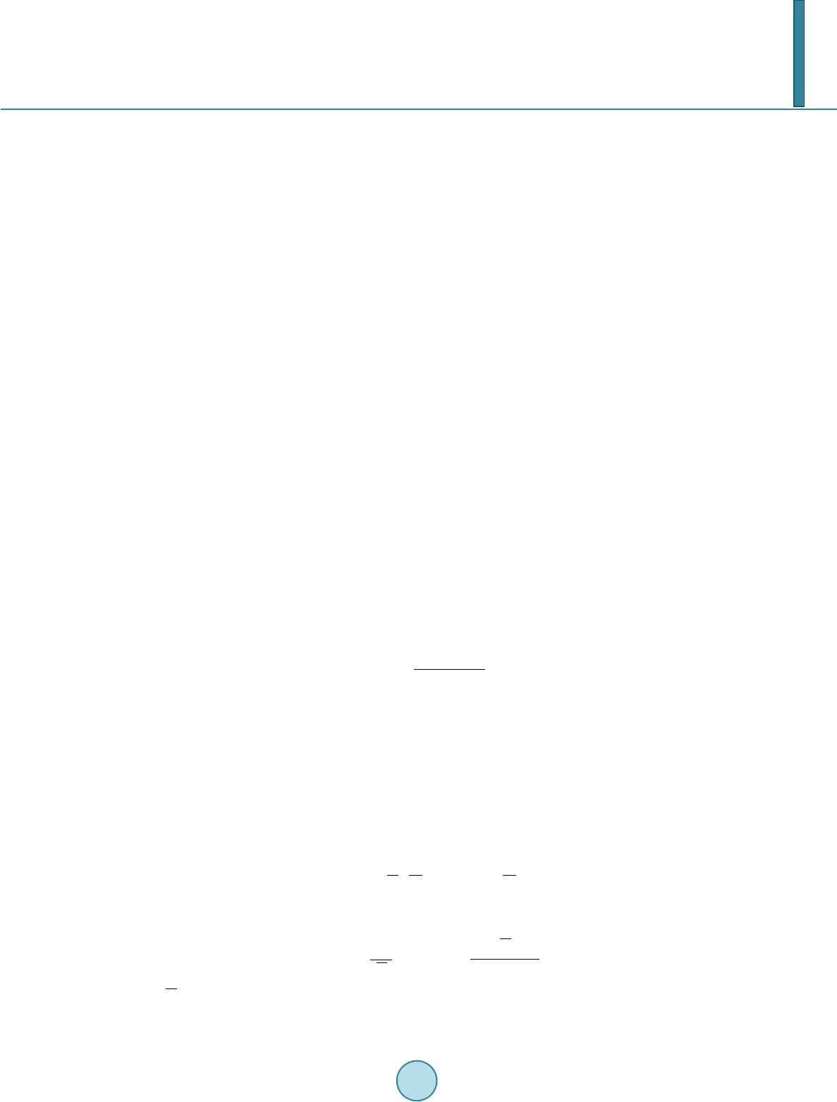
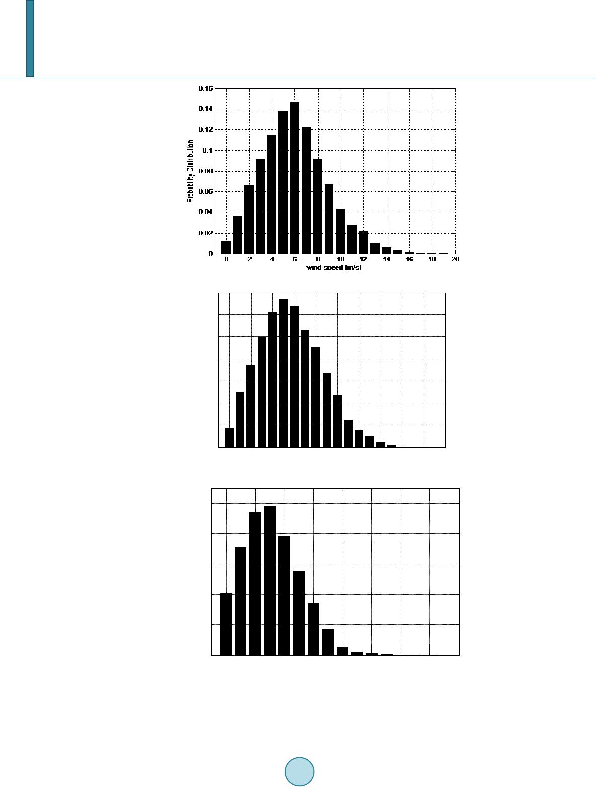
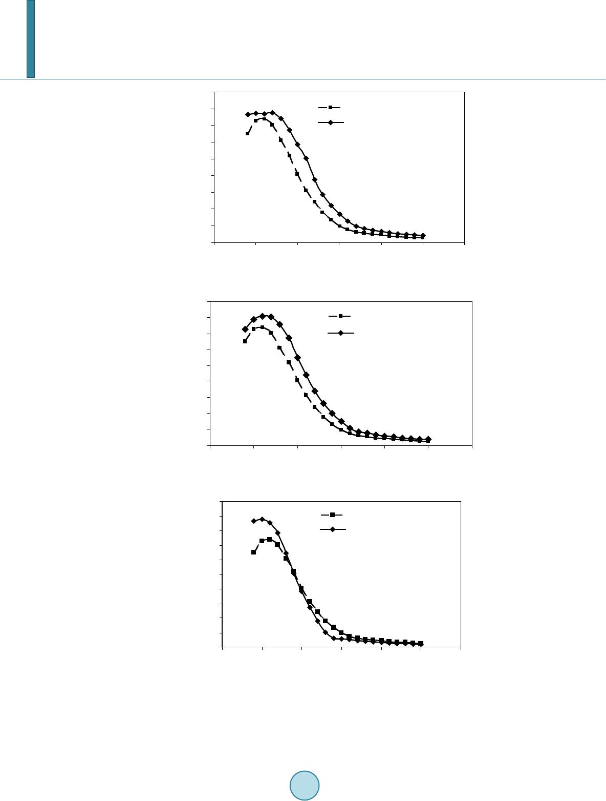
Normally, the design of optimal blade was carried out using one design wind speed. Due to the fact that wind
turbine was operating among fluctuated wind speed at a site. Thus, the pitch regulation was required to optimize
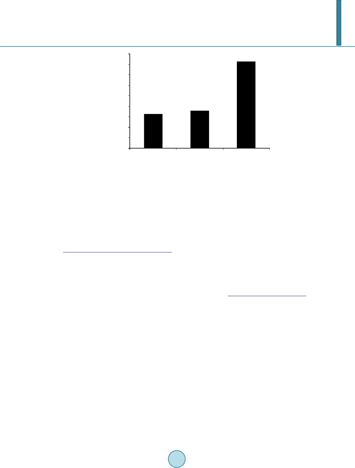
the annual yield for a given wind statistic. As the results, the optimal w in d turbines operated under the three
cases of wind statistic in Nakhonratchasima, Phetchaboon and Ubonratchathani produced the AEP of 52.40,
49.08 and 14.06 MWh at pitch angle of 3˚, 2˚ and 2˚, respectively as shown in Figure 9. Whereas the original
wind turbine produced the AEP of 40.96, 38.52 and 12.51 MWh which were decreased by 28.38%, 35.08 % and
15.96% compare with the optimized results. The results from Table 3 could be summarized that the COE eva-
luated from the optimal wind turbines could be reduced by 13.62%, 10.67% an d 31.83% compare with the orig-
inal results.
As the results, the optimal wind turbine operated under the higher potential sites contributed the greater an-
nual yield which leaded to the lower COE (Figure 10). However, the high profit margin does not only rely on a
W. Sridech, T. Chitsomboon
16
Figure 3. Model of the profile.
(a)
(b)
Figure 4. (a) Comparison of chord distribution; (b) Comparison of
twist angle distribution (Nakhonratchasima).
(a)
(b)
Figure 5. (a) Comparison of chord distribution (b) Comparison of
twist angle distribution (Phetchaboon).
0.4c
0.9t
t
sA
0.2 0.3 0.4 0.50.6 0.7 0.8 0.91
0
0.5
1
1.5
r/R
chord length [m]
original chord
optimized chord
smoothed chord
0.2 0.3 0.4 0.50.6 0.7 0.80.9 1
-10
0
10
20
30
r/ R
twist angle [degree]
original twist
optimized twist
smoothed twist
0.2 0.3 0.4 0.5 0.6 0.7 0.8 0.9 1
0
0.5
1
1.5
r/ R
chord length [m]
original chord
optimized chord
smoothed chord
0.2 0.3 0.4 0.50.6 0.7 0.8 0.91
-10
0
10
20
30
r/ R
twist angle [degree]
original twist
optimized twist
smoothed twist
W. Sridech, T. Chitsomboon
17
Table 3. The optimal thickness and the minimum COE comparison between the optimized and the original wind turbine.
Area Optimal Thickness [mm] COE [$/kWh]
Original Smoothed
Nakhonratchasima 29.23 0.1909 0.1649
Phetchaboon 30.19 0.2025 0.1809
Ubonratchathani 24.38 0.6091 0.4152
(a)
(b)
Figure 6. (a) Comparison of chord distribution (b) Comparison of twist angle distribution (Ubonratchathani).
minimum COE but concerns with a machine rating as well. What if the machine rating is increased, the higher
electricity produced, the higher profitable revenue would be gained accordingly. This issue will be carried out in
the further work.
6. Conclusion
The wind turbines imported from aboard were designed for the windy areas those were not working properly in
the weak w ind areas as in Thailand. Thus, optimizing wind turbine blades for domestic using could be the best
solution for reducing the initial cost and enhancing the performance of wind turbine. As the results, the AEP
produced by the wind turbines optimized with the local wind statistic in Nakhonratchasima, Phetchaboon and
Ubonratchathani were increased by 28.38%, 35 .08 % and 15.96%, respectively whereas th e corr espon d ing COE
have been decreased by 13.62%, 10.67% and 31.83%, respectively. For a long term consideration, it is worthy
of installing these wind turbines because of the enormous profitable revenue from electricity selling corre spond
to the higher AEPs and the lower CO Es can be achieved.
0.2 0.3 0.4 0.5 0.6 0.7 0.8 0.9 1
0
0.5
1
1.5
r/R
chord length [m]
original chord
optimized chord
smoothed chord
0.2 0.3 0.4 0.50.6 0.7 0.8 0.91
-10
0
10
20
30
r/R
twist angle [degree]
original twist
optimized twist
smoothed twist
W. Sridech, T. Chitsomboon
18
(a)
(b)
(c)
Figure 7. The power coefficient, comparison of between the optimized and
the original wind turbine (a) Nakhonratchasima (b) Phetchaboon (c) Ubo-
nratchathani.
0.00
0.05
0.10
0.15
0.20
0.25
0.30
0.35
0.40
0.45
0510 15 20 25 30
Wind speed [m/s]
Cp
Phase VI
Smoothed blade, Tip pitch = 3
0.00
0.05
0.10
0.15
0.20
0.25
0.30
0.35
0.40
0.45
05 10 1520 25 30
Wind speed [m/s]
Cp
Phase VI
Smoothed blade, Tip pitch = 2
0.00
0.05
0.10
0.15
0.20
0.25
0.30
0.35
0.40
0.45
0.50
0510 15 2025 30
Wind speed [m/s]
Cp
Phase VI
Smoothed blade, Tip pitch = 2
W. Sridech, T. Chitsomboon
19
(a)
(b)
(c)
Figure 8. The power curve, comparison between the optimized and the original
wind turbine (a) Nakhonratchasima (b) Phetchaboon (c) Ubonratchathani.
0
2000
4000
6000
8000
10000
12000
14000
16000
18000
0510 15 20 25 30
Wind speed [m/s]
Power [W]
Phase VI
Smoothed blade, Tip pitch = 3
0
2000
4000
6000
8000
10000
12000
14000
16000
0510 15 2025 30
Wind speed [m/s]
Power [W]
Phase VI
Smoothed blade, Tip pitch = 2
0
2000
4000
6000
8000
10000
12000
05 10 1520 25 30
Wind speed [m/s]
Power [W]
Phase VI
Smoothed blade, Tip pitch = 2
W. Sridech, T. Chitsomboon
20
(a)
(b)
(c)
Figure 9. The variation of AEP with pitch angle (a) Nakhonratchasima (b) Phe-
tchaboon (c) Ubonratchathani.
20000
25000
30000
35000
40000
45000
50000
55000
60000
-5 -3 -11357911 13
Tip pitch [degree]
AEP [kW.h/year]
20000
25000
30000
35000
40000
45000
50000
55000
-5 -3-11357911
Tip pitch [degree]
AEP [kW.h/year]
2000
4000
6000
8000
10000
12000
14000
16000
-5 -3-11357911 13
Tip pitch [degree]
AEP [kW.h/year]
W. Sridech, T. Chitsomboon
21
Figure 10. The optimal COE from the three case studies.
Acknowledgements
The authors would like to thank for the data used in this work that has been supported by the Electricity Gene-
rating Authority of Thailand.
References
[1] Spera, D.A. (1994) Wind Turbine Technology: Fundamental Concepts of Wind Turbine Engineering. ASME Press,
New York.
[2] Cartar, J., Ramirez, P. and Velazquez, S. (2008) Influence of the Level of Fit of a Density Probability Function to
Wind-Speed Data on the WECS Mean Power Output Estimation. Energy Conversion and Management, 49, 2647-2655.
http://dx.doi.org/10.1016/j.enconman.2008.04.012
[3] Giguère, P., Selig, M.S. and Tangler, J.L. (1999) Blade Design Trade-Offs Using Low-Lift Airfoils for Stall-Regulated
HAWTs. ASME/AIAA Wind Energy Symposium, Nevada, 11-14 January 1999.
[4] Sridech, W. and Chitsomboon, T. (2008) Optimal Stall-Regulated Wind Turbines in Unique Local Wind Statistic. The
22nd Conference of Mechanical Engineering Network of Thailand, Bangkok.
[5] Benini, E. and Toffolo, A. (2002) Optimal Design of Horizontal-Axis Wind Turbines Using Blade-Element Theory and
Evolutionary Computation. Journal of Solar Energy Engineering, 124, 357. http://dx.doi.org/10.1115/1.1510868
[6] Humtae, C. and Chitsomboon, T. (2012) The Effect of Wind Speed and Wind Statistics Skewed on the Commercial
Wind Turbine in Thailand. The 26th Conference of Mechanical Engineering Network of Thailand, Chengrai.
[7] International Electrotechnical Commission (1998) IEC 61400-1, Ed. 2: Wind Turbine Generator Systems-Part 1: Safe-
ty Requirements. FDIS 1998-12-15.
0.00
0.05
0.10
0.15
0.20
0.25
0.30
0.35
0.40
0.45
Nakhonratchasima
Phe tchaboon
Ubonratchathani
Optimal COE ($/kW.h)