Journal of Geographic Information System, 2011, 3, 99-119
doi:10.4236/jgis.2011.32007 Published Online April 2011 (http://www.SciRP.org/journal/jgis)
Algorithmic Foundation and Software Tools for Extracting
Shoreline Features from Remote S ensing Imagery
and LiDAR Data
Hongxing Liu1, Lei Wang2, Douglas J. Sherman3, Qiusheng Wu1, Haibin Su1
1Department of Ge ography, University of Cincinnati Cincinnati, USA
2Department of Geography & Anthropology Louisiana State University, Baton Rouge, USA
3Department of Ge ography, Texas A&M University College Station, USA
Received January 3, 2011; revised January 8, 2011; accept e d January 12, 2011
Abstract
This paper presents algorithmic components and corresponding software routines for extracting shoreline
features from remote sensing imagery and LiDAR data. Conceptually, shoreline features are treated as
boundary lines between land objects and water objects. Numerical algorithms have been identified and de-
vised to segment and classify remote sensing imagery and LiDAR data into land and water pixels, to form
and enhance land and water objects, and to trace and vectorize the boundaries between land and water ob-
jects as shoreline features. A contouring routine is developed as an alternative method for extracting shore-
line features from LiDAR data. While most of numerical algorithms are implemented using C++ program-
ming language, some algorithms use available functions of ArcObjects in ArcGIS. Based on VB .NET and
ArcObjects programming, a graphical user’s interface has been developed to integrate and organize shoreline
extraction routines into a software package. This product represents the first comprehensive software tool
dedicated for extracting shorelines from remotely sensed data. Radarsat SAR image, QuickBird multispectral
image, and airborne LiDAR data have been used to demonstrate how these software routines can be utilized
and combined to extract shoreline features from different types of input data sources: panchromatic or single
band imagery, color or multi-spectral image, and LiDAR elevation data. Our software package is freely
available for the public through the internet.
Keywords: Shoreline Extraction, Remote Sensing Imagery, LiDAR Data, ArcGIS, ArcObjects, VB.NET
1. Introduction
A shoreline is a spatially continuous line of contact be-
tween the land and a body of water (sea or lake). The
terms “shoreline” and “coastline” are often interchange-
ably used in geosciences and coastal research communi-
ties [1]. It has been long recognized that information
about shoreline position, orientation, and geometric
shape is essential for coastal scientists, engineers and
managers. Depending on the application context, the re-
quirements for shoreline information vary in terms of
shoreline positional accu racy, spatial resolution and cov-
erage, and temporal frequency in survey and mapping. In
the design of shipping structures, coastal defense and
protection infrastructure, coastal en gineers often need the
precise geographical position and detailed shape of sho-
relines within a certain coastal stretch [2]. Coastal man-
agers and land use planners rely on up-to-date shoreline
information at regional scales for establishing legal
property boundary definition and building setback lines
[3,4], estimating recreational beach width and volume [5],
inventorying wetland and agricultural land resources
[6,7], delineating flood and hurricane hazard zones, and
assessing the coastal vulnerability and response man-
agement strategies to climate changes [8-10]. Coastal
scientists and geomorphologists have utilized multi-tem-
poral shoreline data for estimating sediment transport
and budgets [11], examining coastal erosion and accre-
tion [12,13], quantifying historical shoreline retreating or
advancing rates [12,14,15], and assessing sea level rise
and its impacts [16,17].
Traditionally, shorelines depicted on nautical charts

H. X. LIU ET AL. 100
and topographic maps were compiled through visual in-
terpretation of aerial photographs [18]. High resolution
aerial photographs contain details of terrain features, and
shorelines can be observed and delineated with great
precision. In recent decades, new approaches have been
developed for shoreline mapping, including the use of
high-resolution satellite imagery [19], and airborne Li-
DAR technology [20-22]. The era of 1-meter or submeter
satellite imagery such as IKONOS, QuickBird, World-
View and GeoEye, present new and exciting opportuni-
ties for geosciences and coastal research community. The
advent of airborne LiDAR technology offers an alterna-
tive means for mapping coastal topograp hy and shor eline
features with unprecedented accuracy and flexibility.
When the LiDAR data are acquired at a low water level,
it is possible to derive various shoreline indicators with
reference to different tidal datums [22,23]. This repre-
sents a major advantage of the LiDAR data over the re-
mote sensing imagery.
One important technical challenge for shoreline map-
ping is to accurately and efficiently interpret and extract
shoreline features from remote sensing imagery and Li-
DAR data onto a vector representation in a map format.
Traditionally, shorelines were manually delineated with a
pencil on vellum paper overlaid on top of aerial photo-
graphs or traced with a cursor from digital remote sens-
ing images on the computer screen. The manual tracing
method is tedious, subjective, time-consuming, and labor
intensive, contributing to long periods between succes-
sive shoreline maps. In the past decades, a great deal of
research effort has been devoted to the automation of
shoreline extraction from remote sensing data. Lee and
Jurkevich [24] presented an edge detection algorithm for
extracting shorelines from a satellite Synthetic Aperture
Radar (SAR) image. Ryan et al. [25] proposed an image
segmentation approach to the shoreline extraction prob-
lem and tested their method on scanned USGS aerial
photographs. Mason and Davenport [26] employed an
edge detection method with a coarse-fine resolution
processing strategy and applied their app roach to satellite
SAR images. Liu and Jezek [27,28] developed an auto-
mated shoreline extraction method based on a locally
adaptive threshold ing algorithm, and its effectiv eness has
been demonstrated with both optical and radar images. In
recent years, numerical techniques have also been de-
veloped to process LiDAR data for extraction of shore-
lines. Stockdon et al. [29] determined the shoreline posi-
tion by fitting regression lines on cross-shore LiDAR
elevation profiles. The contouring method has been used
by many researchers to derive shorelines from the Li-
DAR data [21,30,31]. Liu et al. [22] developed a seg-
mentation-based method for extracting tidal datum ref-
erenced shorelines from LiDAR data. Despite the pro-
gresses described above, very few studies have been
conducted for a comprehensive analysis and assessment
of algorithmic foundation for extracting shoreline fea-
tures from both remote sensing imagery and LiDAR ele-
vation data. To our knowledge, no dedicated software
tools exist at present for automated shoreline extraction.
Based on our previous research and application ex-
periences [22,23,27,28,32], we made a critical assess-
ment of existing algorithms for sh oreline extraction. This
paper aims to identify the best algorithmic components
for shoreline extraction and to present methods for im-
plementing these algorithms into re-usable software rou-
tines. The algorithms and software routines presented in
this paper are object-based in the sense that shoreline
features are treated as boundary lines between land ob-
jects and water objects. Numerical algorithms are de-
vised and combined to create continuous land and water
objects and then trace the boundaries between land and
water objects into vector shoreline representations. Fur-
ther, an optimized contouring routine is developed as an
alternative approach to shoreline delineation from Li-
DAR data. The software routines and the graphical user’s
interfaces are implemented using the object-oriented
programming (OOP) languages C++ and VB.NET in
conjunction with ESRI ArcObjects. While most core
numerical algorithms are implemented using the compu-
tationally high performance C++ programming language,
some are realized using available functions of Ar-
cObjects in the ArcGIS environment. A graphical user’s
interface has been developed for each routine by pro-
gramming ArcObjects through VB.NET language. Con-
sequently, the software has been integrated as an ArcGIS
extension module named as “ShorelineExtracto r”. In this
paper, Radarsat SAR image, QuickBird multispectral
image, and airborne LiDAR data have been used to illu s-
trate how software routines can b e utilized and co mbined
to automate shoreline extraction from different data
sources: panchromatic or single band imagery, color or
multi-spectral image, and LiDAR elevation data. We
believe that this paper and the corresponding software
package will provide the geosciences and coastal re-
search community with a powerful tool for efficiently
processing high-resolution remote sensing imagery and
LiDAR for frequent and timely shoreline measurements.
2. Algorithmic Foundations for Shoreline
Extraction
Shoreline extraction from imagery is a complicated
process. Because of frequent lack of sufficient contrast
between the land and water bodies on images and the
difficulty in distinguishing shoreline features from other
linear features, most general-purpose algorithms for edge

H. X. LIU ET AL.101
and linear feature detection are not adequate for the
automated coastline extraction. Previously, two ap-
proaches have been employed for shoreline extraction
from images. One approach treats shoreline extraction as
an edge detection problem. This approach is based on the
observation that image intensity (gray) values across the
shoreline change abruptly, so that spatial differentiation
operators and edge detectors may be used to locate
meaningful intensity variations and discon tinuities on the
image as candidate shoreline pixels. The other approach
treats the shoreline as the boundary between two rela-
tively homogeneous objects (land and water objects),
each with a distinct average intensity value. The
edge-based approach suffers from the fact that the edge
pixels produced by edge detectors are often discontinu-
ous and seldom characterizes a shoreline completely
[24,26,28]. To assemble and link edge pixels separated
by small breaks is a computationally in tensive task, even
for a crude approximation [24,33]. In contrast, the ob-
ject-based approach has the advantage of creating a con-
tinuous boundary between the land and water objects
[23,28]. Therefore, we adopt the object-based approach
for the development of shoreline extraction algorithms
and software routines for image data.
Different from remote sensing imagery, the LiDAR
data are elevation measurements rather than the reflected
intensity of radiation. The shorelines cannot be visually
interpreted from LiDAR data, but can be inferred from
the elevation values with reference to a tidal datum. We
adopt two approaches to the processing of LiDAR data
for shoreline extraction. The first is object-based, similar
to the one u sed for process ing image data. By comparing
the LiDAR DEM with the tidal datum surface, grid
cells/pixels with an elevation value higher than the tidal
datum can be grouped into land objects, while grid
cells/pixels with an elevation below the tidal datum can
be grouped into water objects. The second approach is
contouring-based. The idea is that after the LiDAR ele-
vation values are adju sted with reference to a tidal da tum,
the grid cells/pixels on the shoreline should assume a
value of zero. Thus, the shorelines can be derived by
contouring zero elevation pixels.
As indicated above, the object-based approach is ap-
plicable to both remote sensing image data and LiDAR
elevation data. This approach is implemented with four
groups of algorithms and software routines: preprocess-
ing, land/water segmentation, object post-processing, and
shoreline generalization. With the object-based approach,
algorithms and software routines used for processing
image data and LiDAR data are almost the same, except
for those used for land/water segmentation. The pre-
processing algorithms aim to suppress data noise and
enhance the contrast between land and water bodies. The
segmentation algorithms partition an image into homo-
geneous land and water objects. The post-object proc-
essing algorithms are designed to differentiate the shore-
line features from other linear features, and trace the
shoreline pixels into a vector representation. The con-
touring based appro ach is only applicable to LiDAR d ata.
This approach consists of three groups of algo rithms and
software routines: preprocessing, shoreline contouring
with a specified reference tidal datum, and shoreline
generalization. Our goal is to create an effective, opera-
tional software tool that minimizes operator’s interven-
tion and editing efforts and maximizes the reliability,
repeatability, and accuracy of the derived shoreline fea-
tures.
We have identified a sequence of key algorithm ele-
ments and implemented 14 software rou tines to auto mate
the coastline extraction process (Figure 1). The shoreline
extraction process can be decomposed into a sequence of
processing tasks. The combination of these routines is
capable of processing panchromatic/single band images,
color/multi-spectral band images, and LiDAR elevation
data for shoreline extraction. Each application scenario
requires a different set of routines as described in the
following section. We implemented the key algorithms
as a series of re-usable DLLs (Dynamic-Link Library)
using the computationally high performance language
C++.NET. These re-usable algorithm components (DLLs)
can be easily incorporated into commercial or open
source GIS and remote sensing software packages as a
plug-in component, including the open source GIS soft-
ware-GRASS, the proprietary GIS software-ArcGIS, and
the proprietary remote sensing software-ENVI.
Considering the widespread use of ArcGIS software
packages in geosciences and coastal research communi-
ties, in this research we select to seamlessly embed our
shoreline extraction software routines into ArcGIS as an
extension module. The combination of the specialized
shoreline extraction programs with ArcGIS as a single
integrated software package allows users to take advan-
tage of the powerful ArcGIS functions in data manage-
ment, visualization, and spatial analysis during the
shoreline extraction process. In this way, the input im-
ages and LiDAR elevation data in ArcGIS compatible
format can be directly loaded in the shoreline extraction
module. Intermediate processing results can be immedi-
ately displayed and checked by using the variety of Ar-
cGIS visualization functions. The shorelines extracted
from remote sensing data are output in ArcGIS data for-
mats and can be further edited and validated using the
ArcGIS’s editing capabilities. Using ArcGIS spatial
analysis functions, final shoreline products can be readily
compared and integrated with other data layers for map
composition and change analysis.

H. X. LIU ET AL. 102
Figure 1. Structure and software routines for shoreline ex-
traction.
We constructed the shoreline extraction extension
module using ArcObjects, which are a set of platform
independent software components designed by ESRI Inc.
specifically for developing ArcGIS applications. We
choose VB.NET to program ArcObjects for creating the
shoreline extraction extension module. The use of
VB.NET makes it easier to package and deploy the ex-
tension module. In addition, it is possible to make the
extension module as a standalone application running
outside ArcGIS using ESRI’s map control. Our extension
module can be wrapped and distributed as a single pack-
age and installed with a user friendly setup procedure.
After installation, the shoreline extraction extension
module appears in ArcGIS as shown in Figure 2.
For each software routine, we devise its graphical in-
terface through a VB.NET program that calls and wraps
the relevant ArcObjects and our specialized DLLs de-
veloped using C++ language. The graphical interface for
each routine is a customized dialogue menu that guides
the user to load the input data, to set the relevant pa-
rameter values, and to specify the outputs. This elimi-
nates the needs for the user to remember the command
syntax and relevant parameter values.
3. Algorithm Components and Software
Routines
Our shoreline module is capable of handling various
types of remote sensing images and LiDAR elevation
data. The commonly used remote sensing image sources
for shoreline mapping include panchromatic aerial pho-
tographs, natural color aerial photographs, near infrared
color aerial photographs, panchromatic satellite images,
multi-spectral satellite images, and synthetic aperture
radar (SAR) images. The input images need to be geo-
referenced and orthorectified b efore the shoreline extrac-
tion operation. The LiDAR data need to be prepared in a
raster grid format and be vertically referenced to a tidal
datum surface in order to derive tide coordinated shore-
line. In the following sections, we describe algorithms
and routines implemented in our extension module, with
the emphasis on the technical improvements.
3.1. Algorithms and Routines for Preprocessing
The purpose for preprocessing the images and LiDAR
data is to reduce data noise and enhance the contrast be-
tween land and water masses for shoreline ed ge detection .
The noise in images and LiDAR data can result in nu-
merous isolated, small, insignificant or spurious edges
other than real shoreline features. This imposes great
complications in subsequent image processing. To ad-
dress the noise issue, we select and implement several
specific noise-reduction filters from the filters published
in the literature. For the shoreline extraction purpose, th e
filters used in the preprocessing stage should have an
edge-preserving property, namely, the ability to remove
data noise while preserving the precise position of shore-
line edges. We select and implement four of such filters
for handling different types of inp ut data: Gau ssian filter,
Lee Sigma filter, median filter, and anisotropic diffusion
operator. It should be noted that although the mean (av-
erage) filter is widely available, it should not be used in
the shoreline extraction process because the use of the
mean filter blurs the land-water boundary edges and in-
creases the shoreline positional error.
1) Gaussian filter: it uses a weight kernel that repre-
sents the shape of a Gaussian (bell-shaped) hump and
outputs a weighted average of pixels in the kernel
neighborhood, with a higher weight assigned to pixels
closer to the central pixel. The Gaussian filter provides
gentle smoothing of data noise without seriously blurring
of major edge features. We implement the Gau ssian filter
through a VB.NET program to call ArcObjects and in-
voke C++ programs. The Gaussian filter is applicable to
both optical images and LiDAR data. Two parameters,
the window size and the standard deviation of the Gaus-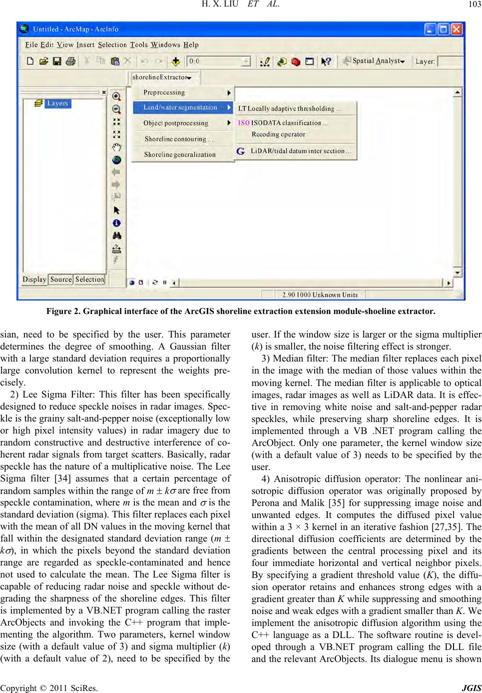

H. X. LIU ET AL. 103
Figure 2. Graphical interface of the ArcGIS shoreline extraction extension module-shoeline extractor.
sian, need to be specified by the user. This parameter
determines the degree of smoothing. A Gaussian filter
with a large standard deviation requires a proportionally
large convolution kernel to represent the weights pre-
cisely.
2) Lee Sigma Filter: This filter has been specifically
designed to reduce speckle noises in radar images. Spec-
kle is the grainy salt-and-pepper noise (exceptionally low
or high pixel intensity values) in radar imagery due to
random constructive and destructive interference of co-
herent radar signals from target scatters. Basically, radar
speckle has the nature of a multiplicative noise. The Lee
Sigma filter [34] assumes that a certain percentage of
random samples within the range of m  k  are free from
speckle contamination, where m is the mean and  is the
standard deviation (sigma). This filter replaces each pixel
with the mean of all DN values in the moving kernel that
fall within the designated standard deviation range (m 
k  ), in which the pixels beyond the standard deviation
range are regarded as speckle-contaminated and hence
not used to calculate the mean. The Lee Sigma filter is
capable of reducing radar noise and speckle without de-
grading the sharpness of the shoreline edges. This filter
is implemented by a VB.NET program calling the raster
ArcObjects and invoking the C++ program that imple-
menting the algorithm. Two parameters, kernel window
size (with a default value of 3) and sigma multiplier (k)
(with a default value of 2), need to be specified by the
user. If the window size is larger or the sigma multiplier
(k) is smaller, the noise filtering effect is stronger.
3) Median filter: The median filter replaces each pixel
in the image with the median of those values within the
moving kernel. The median filter is applicable to optical
images, radar images as well as LiDAR data. It is effec-
tive in removing white noise and salt-and-pepper radar
speckles, while preserving sharp shoreline edges. It is
implemented through a VB .NET program calling the
ArcObject. Only one parameter, the kernel window size
(with a default value of 3) needs to be specified by the
user.
4) Anisotropic diffusion operator: The nonlinear ani-
sotropic diffusion operator was originally proposed by
Perona and Malik [35] for suppressing image noise and
unwanted edges. It computes the diffused pixel value
within a 3 × 3 kernel in an iterative fashion [27,35]. The
directional diffusion coefficients are determined by the
gradients between the central processing pixel and its
four immediate horizontal and vertical neighbor pixels.
By specifying a gradient threshold value (K), the diffu-
sion operator retains and enhances strong edges with a
gradient greater than K while suppressing and smoothing
noise and weak edges with a gradient smaller than K. We
implement the anisotropic diffusion algorithm using the
C++ language as a DLL. The software routine is devel-
oped through a VB.NET program calling the DLL file
and the relevant ArcObjects. Its dialogue menu is shown

H. X. LIU ET AL. 104
in Figure 3(a). The two parameters, the gradient thresh-
old (K) (with a default value of 8) and the iteration num-
ber (with a default value of 5), need to be specified by
the user. The larger the gradient threshold value or the
iteration number, the stronger the smoothing effect. The
appropriate choice of the gradient threshold value can
achieve the intended objective of enhancing the major
edges along the shoreline features while suppressing
noise, interior variations, and unimportant weak edges
inside land or water objects [27].
Figure 3. Graphical interfaces for selected shoreline extraction routines. (a) anisotropic diffusion routine; (b) locally adaptive
thresholding routine; (c) ISODATA classification routine; (d) LiDAR/tidal datum intersection; (e) morphology operator rou-
ine; (f) object formation and removal routine; (g) shoreline contouring routine; and (h) shoreline generalization. t

H. X. LIU ET AL. 105
3.2. Algorithms and Routines for Segmenting
and Classifying Land and Water Pixels
Forming homogenous land and water objects for shore-
line extraction requires an accurate and reliable differen-
tiation of land pixels from water pixels. The border pix-
els between segmented land/water objects can be then
delineated as the shorelines. The separation of an image
or a LiDAR DEM into constituent land and water parts is
the most important step in the object-based approach.
Three algorithms and software routines are implemented
for this purpose. Those include the locally adaptive
thresholding, ISODATA classification followed by a
recoding operation, and intersection of LiDAR grid and
the selected tidal datum. The locally adaptive threshold-
ing routine is designed to segment a panchromatic or
single band image into land and water pixels. The ISO-
DATA classification routine can classify a color or
multi-spectral imagery into a number of land cover clus-
ters, which can be subsequently combined into two
categories (land and water pixels) through the recoding
routine. The LiDAR grid and tidal datum intersection
routine compares LiDAR elevation values with the cor-
responding tidal datum values and classify LiDAR ele-
vation grid cells into land and water pixels.
1) Locally adaptive thresholding: it is the key algo-
rithm component for segmenting a panchromatic or sin-
gle band image into land and water pixels. The underly-
ing concept is that the histogram of a small image region
that contains a shoreline can be characterized by a mix-
ture of double Gaussian distributions. First, the entire
image is subdivided into a set of small, overlapping,
square regions. For each small region, we examine the
bi-modality and analytically determine a local threshold
value to separate the land p ixels from the water pixels. If
the small image region consists solely of land or water
pixels, the probability distribution of the intensity values
will be uni-modal. If the image region consists of both
land and water pixels, namely, the region contains shore-
line features, the intensity values of land pixels and water
pixels will be grouped into two dominant modes
(bi-modality) with distinct mean values. The overall his-
togram for this region would exhibit two peaks and a
valley. The lowest histogram valley point is used as a
threshold value to reliably classify the pixels into land
and water pixels.
To computationally determine the valley point, the
bimodal histogram is modeled with a mixture of two
Gaussian (normal) distribution functions, in which there
are five unknown parameters to be determined [28,36].
The Levenberg-Marquardt algorithm is used to itera-
tively compute the optimal estimates for the five pa-
rameters based on the observed histogram [28], and op-
timal threshold value can be computed analytically.
For all the small image regions whose histograms have
appreciable bi-modality [28,36], optimal local thresholds
can be computed using the process described above. As a
result of processing all the image regions, a set of ir-
regularly distributed threshold values are obtained. Next,
an Inverse Distance Weighted (IDW) interpolation
method [28] is employed to interpolate these irregularly
distributed threshold values into a threshold grid. In other
words, a threshold value is estimated for every pixel
based on the threshold values of adjacent image regions
using spatial interpolation. Subsequently, all the image
pixels are segmented into land and water pixels by com-
paring their intensity values with corresponding local
threshold values. If a pixel has an intensity value above
its local threshold, it is flagged as a land pixel. Otherwise,
it is designated as a water pixel. The locally adaptive
thresholding algorithm can be summarized into the fol-
lowing computational steps:
1) Divide the input image into a set of small, overlap-
ping, square image regions;
2) Construct an observed histogram for each image re-
gion, and optionally smooth the histogram using a one-
dimensional Gaussian filter;
3) Estimate initial values for the five parameters of the
bimodal Gaussian curve and use the Levenberg-Mar-
quardt algorithm to iteratively fit the bimodal Gaussian
parameter s for e ac h re gion;
4) Test the resulting Gaussian curve for bi-modality;
5) Based on the fitted estimates for the five bimodal
Gaussian parameters, calculate the optimal local thresh-
old for any region whose histogram passes the bi-mo-
dality test;
6) Repeat steps (2)-(5) until all image regions are
processed;
7) Interpolate local thresholds into a threshold grid
with the IDW algorithm; and
8) Segment the entire image into land or water pixels
by comparing the intensity values with their local thresh-
old value s.
If a single global threshold were used for the entire
image, some shoreline edges would remain undetected
due to the heterogeneity of the intensity contrast, cau sing
discontinuous shoreline edges in low contrast areas and
inconsistency of shoreline edge positions between high
contrast and low contrast areas [28]. Since the locally
adaptive thresholding algorithm sets the threshold value
dynamically according to the local image statistical
properties, a good separation between the land and water
can be achieved.
We implement the locally adaptive thresholding algo-
rithm using the C++ language as a DLL. A VB.NET
program is written to call this DLL and relevant Ar-

H. X. LIU ET AL. 106
cObjects for the development of a graphical interface.
The dialogue menu is shown in Figure 3(b). Two critical
parameters need to be specified by the user for this rou-
tine. One is the width of the squ are image region s u sed to
subdivide the image. The width of the regions is speci-
fied in pixels with a default value of 32. The width
should be small enough so that only one or two catego-
ries of pixels exist in the region. It also should be big
enough to ensure reliable statistical analysis of the histo-
gram. Normally, the larger the width, the more general-
ized the resulting land and water objects. The other pa-
rameter is the bi-modality criterion indicated by a mini-
mum value of the valley/peak ratio (valley height/lower
peak height). Optimal local threshold values would be
analytically determined only for those image regions
whose histograms have a valley/peak ratio larger than the
minimum value. The default value for the bi-modality
criterion is set as 0.8. A lower criterion value will result
in fewer but more reliable optimal thresholds to b e com-
puted. The smoothing of the histogram can speed up the
convergence of the iterative computation of the Leven-
berg-Marquardt algorithm, if the image is noisy. Whether
or not to smooth the observed histogram for each image
region is controlled by a check button on the dialogue
menu.
2) ISOADATA classification and recoding operator:
The Iterative Self-Organizing Data Analysis Technique
(ISODATA) [37] is a popular unsupervised classification
method. With the ISODATA classification algorithm, a
color or multi-spectral remote sensing image can be clas-
sified into a number of surface cover types, which can be
further merged into two broad categories, land and water
pixels, by using a recoding operator.
ISODATA classification performs an iterative, opti-
mization clustering of a multi-spectral image. First, it
arbitrarily assigns initial mean values for a specified
number of clusters with equal interval that is defined by
the mean and standard deviation of each band of the
multi-spectral image. The region in the spectral space is
defined using the mean and standard deviation of each
band. In the first iteration, the multi-spectral values of
each candidate pixel are compared to the mean values of
different spectral bands of each cluster. The Euclidean
distance between the multi-spectral values of each pixel
and the mean values of each cluster is calculated. The
candidate pixel is assigned to the cluster whose Euclid-
ean distance is the shortest from the pixel. In the second
iteration, new mean values are re-calculated for all the
spectral bands of each cluster based on the pixels actu-
ally assigned to each cluster using the minimum Euclid-
ean distance rule in the first iteration. The formed clus-
ters are then diagnosed to decide whether or not they
need to be merged or split. If a cluster contains less than
the minimum percentage of pixels, it would be merged
with the nearest cluster. If the Euclidean distance be-
tween the mean values of two clusters is below a thresh-
old (default value of 3), these two clusters will be
merged. If the standard deviation for a cluster exceeds a
specified maximum standard deviation (typically be-
tween 4.5 and 7) or the number of pixels in a cluster is
greater than the specified maximum number, the cluster
will be split into two clusters. Mean values for the two
new clusters are calculated as the mean of the original
single cluster plus or minus the standard deviation. After
the merging and splitting process, the mean values for
new clusters are calculated. In the next iteration, every
pixel in the image is once again assigned to a cluster us-
ing the minimum Euclidean distance rule. This iterative
process is repeated until there is little change in class
assignment between iterations or the maximum number
of iterations is reached. At the final iteration, pixels are
assigned to clusters using a maximum-likelihood deci-
sion rule based on the means and standard deviations of
the spectral bands of each cluster.
We implement the ISODATA classification algorithm
through a VB.NET program calling the available func-
tions of ArcObjects. The dialogue menu for this routine
is shown in Figure 3(c). Four parameters need to be set
to run this routine: the number of output clusters, the
number of iterations, minimum cluster size in pixel, and
sample interval in pixel. The specified number of clusters
(default value is 3) is the maximum number of clusters to
be identified in the iterative clustering process. It is ad-
vised to enter a conservatively high number, analyze the
resulting clusters, and to then re-run the function with a
reduced number of classes. The number of the iterations
(the default is 20) specifies the number of rounds to clas-
sify pixels and recalculate cluster mean values. The
ISODATA algorithm terminates when this number is
reached. This number should be large enough to ensure
that after running the specified number of iterations, the
migration of pixels from one cluster to another is mini-
mal, and the clusters have become stable. Minimum
cluster size (the default is 20) specifies the number of
pixels to form a valid cluster, and clusters containing
pixels fewer than this number will be merged with other
clusters. This minimum cluster size should be about 10
times larger than the number of bands in the
multi-spectral imagery in order to obtain reliable statis-
tics. The sample interval (the default is 10) specifies the
row and column interval between pixels that are actually
sampled and used in the iterative computation of the
mean and standard values of the spectral bands of the
clusters. Larger sample intervals reduce the computation
time but may introduce bias in the statistics.
The output of ISODATA routine is a classified image,

H. X. LIU ET AL.107
and each pixel has an integer value to indicate the identi-
fication number of each cluster. A recoding routine is
developed using a VB.NET program calling the relevant
ArcObjects. The recoding routine can load and display
the classified image from the ISODATA classification,
and on the dialogue menu the user can specify which
clusters should be categorized as land pixels and which
as water pixels through visual inspection of the classified
image. Therefore, the combination of ISODATA classi-
fication and the recoding operation creates a binary im-
age consisting of land and water pixels.
3) LiDAR/tidal datum intersection: This routine aims
to segment LiDAR elevation grid cells into land an d wa-
ter pixels by comparing the elevations with a tidal datu m
value. If a pixel has an elevation lower than the tidal da-
tum value, it is coded as a water pixel. Otherwise, it is
coded as a land pixel. Th e LiDAR elevation grid and the
tidal datum grid must be referenced to a common datum
[22]. This routine is implemented through a VB.NET
program calling relevant ArcObjects. On the dialogue
menu for th is ro u tin e ( Figure 3(d)), the input tidal datum
surface can be specified as a constant value or loaded as
a grid with varying values. For a small study area, the
tidal datum can be treated as a constant valuable obtained
from the nearest tidal gauge station. For a large study
area, a tidal datum grid should be created by interpolat-
ing the tidal datum values measured by all tidal gauge
stations in the study area.
3.3. Algorithms and Routines for
Post-Processing Land and Water Objects
As described above, we can obtain a classified binary
image consisting of land and water pixels by applying
locally adaptive thresholding routine to a panchromatic
or single band image, or by applying the ISODATA
classification to a color or multi-spectral image followed
by the recoding operation, or by intersecting a LiDAR
DEM with a tidal datum surface. In the binary image,
spatially connected land pixels form homogenous land
objects, and spatially connected water pixels constitute
homogeneous water objects. Misclassifications may oc-
cur, due to data noise, insufficient or inconsistent con-
trast between land and water, and the complexity of the
scene. For instance, wet surfaces, cloud shadows, and
building shadows are often misclassified as water objects,
and whitewater, foam, ships, oil rigs, and clouds are of-
ten misclassified as land objects. The primary character-
istic of these misclassified objects is that their areal size
is significantly smaller than that of true land or water
objects. To correct misclassifications and achieve a reli-
able shoreline, land and water objects need to be further
processed before extracting the boundaries as shorelines.
Three software routines are devised to achieve this goal:
morphology operator, object identification and spurious
object removal, and object boundary tracing. The mor-
phology operator [38,39] aims to smooth the boundaries
of land and water objects. The object identification and
spurious object removal routine is intended to explicitly
form image objects and then eliminate misclassified and
unwanted objects. The object boundary tracing routine is
used to delineate the boundaries between land and water
objects as shoreline features and output them as ArcGIS
vector data (ERSI Shape files or geodatabase feature
class).
1) Morphology operator: Because of data noise and
resolution limitation, land and water objects created in
the segmentation and classification stage often exhibit
noisy and jagged boundaries. Many tiny inlet- and pen-
insular-like features along the boundaries are spurious.
The morphology operator is designed to smooth the
boundaries and eliminate erroneous small-scale inlet-
and peninsular-like features. The morphology operator is
based on two fundamental operations: dilation and ero-
sion [33,38,39]. Dilation adds pixels to the perimeter of
each image object, generally increasing the size of ob-
jects, thus potentially filling small holes and broken areas,
and connecting disjoint objects that are separated by
spaces smaller than the size of the structuring element.
Erosion etches pixels away from the perimeter of each
image object and therefore shrinks the object. The opera-
tions of dilation and erosion can be combined into more
complex sequences. The most useful combinations for
morphological filtering are known as opening and clos-
ing. Opening consists of an erosion followed by a dila-
tion and can be used to eliminate all pixels in regions that
are too small to contain the structuring element. Closing
consists of a dilation followed by erosion and can be
used to fill in holes and close small gaps. We implement
the morphology operator using the C++ language as a
DLL. A VB.NET program is developed to call this DLL
and relevant ArcObjects. The dialogue menu for this
routine is shown in Figure 3(e). Closing, opening, and
any sequential combination of dilation and erosion op-
erations can be specified on this menu. In addition, two
simple morphology operations, fill and trim, are also
added as alternative option s on the menu. The fill op era-
tion fills single-pixel interior holes or single-pixel dents
and cavities on the boundary. The trim operation cuts off
single pixel protrusions and overhangs on the boundary.
2) Object formation and spurious object removal: The
fundamental observation is that real land and water
(ocean) masses usually form large, continuous image
objects. Erroneous and misclassified image objects
commonly have a significantly smaller size. Explicitly
grouping connected land and water pixels into individual

H. X. LIU ET AL. 108
image objects and deriving their geometric properties
renders the capability of discriminating erroneous and
misclassified objects from true land and water objects
based on the heuristic knowledge about the size and con-
tinuity of land and water bodies in the stud y area. A land
object consists of a set of sp atially connected land pixe ls.
Two land pixels are defined to be connected if one is
located in the immediate neighborhood of the other. A
recursive expansion algorithm is used to identify and
index image objects [28,33]. First, the image is scanned
in a row-wise manner, and a seed is set at the first land
pixel, which is treated as a single pixel land object. This
single pixel object is expanded to include all land pixels
located in the immediate neighborhood of the current
land pixel. The expansion is continued recursively until
all connected land pixels are included. This recursive
expansion process may be repeated to identify other land
objects. The land objects are indexed with a unique inte-
ger, starting with 1. During the object formation and in-
dexing process, the areal size and other geometric prop-
erties of each object are also calculated. Small non-water
objects scattered in the water bodies often correspond to
ships, oil rigs, ice bergs, clouds, whitewater, foam, or
image noise. Since the boundaries of these small image
objects are not true shorelines, they should be selected
with an area threshold and eliminated by fusing them
into the water bodies. Similarly, water objects can be
explicitly identified and indexed, and small noisy water
objects corresponding to wet surfaces, building and
cloud shadows, and data noise can be dissolved into the
land with another user specified areal threshold value.
We implement the object identification and spurious
object removal routine using the C++ language as a DLL.
The software routine is developed through a VB.NET
program invoking the DLL and calling ArcObjects. The
dialogue menu for this routine is shown in Figure 3(f).
The user needs to specify the object value and back-
ground value. The parameter of the areal size threshold
value in pixel needs to be specified by the user to remove
small noisy image objects. In practice, this routine is run
in two passes. Assume that in a segmented image the
land pixels are coded by the value of 255 and water pix-
els are coded by the value of 0. In the first pass, by
specifying the object value to be 255 and background
value to be 0, land objects are identified and spurious
objects specified by the size threshold value are removed.
In the second pass, by specifying the object value to be 0
and the background value to be 255, water objects are
identified and small water objects specified by the size
threshold value are eliminated. After two passes of selec-
tive removal of small, isolated, and noisy image objects,
only large continuous land and (ocean) water objects are
left, which define true shorelines. This routine can effec-
tively eliminate unwanted, misclassified objects whose
boundaries are not shorelines. This greatly reduces the
editing cost for cleaning up the final shoreline product.
3) Boundary tracing and vectorization: with the object
based approach, the shoreline is defined as the boundary
between land and water objects. Each land pixel in an
image object is scanned by a 3 × 3 neighborhood win-
dow to examine its four immediate neighbors (horizontal
and vertical). If one or more neighbors of the land pixel
belong to water (background) pixels, this land pixel will
be flagged as a boundary pixel. In this way, all land pix-
els immediately adjacent to the water pixels are extracted
as boundary pixels. Then, a recursive algorithm is used
to trace boundary pixels into a set of vector lines. The
output of this routine is an ArcGIS Shape file containing
vector shorelines, which can be directly displayed, vali-
dated and edited in the ArcGIS environment.
3.4. Algorithm and Routine for Contouring
LiDAR Data for Shorelines
Shorelines can be derived from LiDAR data alternatively
by using a contouring method. First, the LiDAR data
need to be adjusted with reference to the tidal datum
surface. After subtracting the tidal datum from the Li-
DAR DEM, the resulting zero elevation cells can be
contoured to represent the tidal-datum referenced shore-
lines. Although the contouring routine is available in
most GIS software packages, it is designed for a general
topographical mapping purpose. To use such a routine,
the user has to specify a base contour line and contour
interval, resulting in a series of contour lines with incre-
mental elevation values. Since these contouring routines
are not optimized for shoreline extraction, they often
produce many short, broken, and noisy shoreline seg-
ments when applied to LiDAR data [21,30,31]. There-
fore, a great deal of manual editing or re-digitizing work
was involved in creating the final clean shoreline repre-
sentation [21,30,31].
To overcome the difficulties, we develop a dedicated
contouring routine for shoreline extraction. This routine
only traces connected cells with a specified elevation
value (zero in most cases). A constraint on the length of
the traced shoreline segments is also imposed for the
contouring process. Noisy and broken dangle lines will
be dropped automatically as long as their length is
shorter than a user specified threshold value. We develop
this software routine using the VB .NET to call Ar-
cObjects. The dialogue menu for this routine is shown in
Figure 3(g). Two parameters can be specified by the
user. One is the elevation to be contoured, and its default
value is zero. The other one is the minimum length of
shorelines to be kept. The output of this routine is a

H. X. LIU ET AL.109
shape file of shorelines, which can be display and edited
further in ArcGIS.
3.5. Algorithms and Routines for Shoreline
Generalization
Two algorithm options are included in the shoreline
smoothing and generalization routine. The first is the
Douglas-Peucker algorithm for line simplification. It
keeps the critical points that depict the essential shape of
the shoreline and removes redundant details such as ex-
traneous bends, fluctuations, small intrusions and extru-
sions. The algorithm connects the end-nodes of a curve
segment with a trend line. The distance of each vertex to
the trend line is measured perpendicularly. Vertices with
a distance to the line less than the specified tolerance are
eliminated. The algorithm is efficient for data compres-
sion, but the resultant shorelines may contain unpleasant
sharp angles and spikes which reduce the cartographic
quality. The second algorithm si mplifies the b ends on the
shorelines. It analyzes the shape of the shorelines and
identifies the high-curvature bends. Insignificant extra-
neous bends are then removed, and too narrow bends are
slightly widened to satisfy the tolerance. Compared with
the Douglas-Peucker algorithm, the bend simplification
algorithm tends to produce smoother and hence carto-
graphically more appealing shorelines. We implement
this software rou tine through a VB.NET program calling
the ArcObjects. Through the dialogue menu, the user can
make a selection between the Douglas-Peucker algorithm
and the bend simplification algorithm. The only parame-
ter that the user needs to sp ecify is the weeding tolerance
value, which determines th e degree of generalization.
4. Shoreline Extraction Scenarios
4.1. Data Sources and Application Requirements
From the data processing perspective, the possible input
remote sensing data for shoreline extraction can be
grouped into three categories: single band imagery, mul-
ti-band imagery, and LiDAR DEMs. The single band
imagery can be panchromatic image, near infrared image,
and Synthetic Aperture Radar image acquired by satellite
or airborne sensors. Multi-band imagery can be natural
color image, false color near infrared image, multi-spec-
tral image, multi-polarimetric SAR image from satellite
or airborne sensors.
In practice, the choice of data sources for shoreline
mapping at a specific site is often dictated by the avail-
ability and cost o f data. The land cover types in the coast
zone and the requirements for spatial coverage and reso-
lution of shoreline also influence the data selection. Al-
though relatively small coastal areas are involved, most
of coastal engineering applications require highly de-
tailed and precise shoreline information, which can be
only satisfied by aerial photograph s in the past. The suc-
cessful launches of IKONOS satellite in September 1999,
QuickBird satellite in October 2001, WorldView-1 satel-
lite in September 2007, and GeoEye-1 Satellite in Sep-
tember 2008 have produced 1-meter or sub-meter satel-
lite imagery, which can be used for high resolution
coastal mapping applications. For coastal resource in-
ventory and management, flood and hazard zone delinea-
tion, and other environmental applications, satellite im-
ages at fine or moderate spatial resolution, such as
Landsat, SPOT, ASTER, and Radarsat SAR images, can
be a good choice due to their extensive ground coverage
and the repetitive acquisition. Coastal erosion and his-
torical shoreline change studies require multi-temporal
shoreline information. Historical data are limited or
nonexistent at the great majority of coastal sites. Satellite
image data did not exist until 1970s, while aerial pho-
tography began to be available for many areas of the
coast in the 1940s [1,40], which is the most common
data source for determining past shoreline positions. For
coasts with sandy beaches or exposed rocks, all types of
image data are applicable for discerning and mapping
shoreline features. For shallow coastal waters with high
concentration of suspended sediments or underwater
features, shorelines can be mapped more easily and ac-
curately from near infrared images and radar images than
from panchromatic and natural color images, because the
land-water contrast is much stronger on the infrared and
radar images. For the low-lying coasts with wetlands,
mangroves and other types of vegetation, the use of color
near infrared aerial photographs and multispectral satel-
lite images would make the separation of water from
land easier and more accurate, with a result of better de-
termination of shoreline position.
Airborne LiDAR promises an accurate and cost-ef-
fective approach to coast and shoreline mapping [20,21].
Airborne LiDAR data have been increasingly available
for the coastal applications since 1990s. The NOAA
Coastal Services Center (CSC) has collected topog-
raphical LiDAR data at 1 m - 2 m resolution along the
United States coasts through a partnership program with
the USGS Center for Coastal and Regional Marine Stud-
ies and the NASA Goddard Space Flight Center
(http://www.csc.noaa.gov/crs/tcm/missions.html). For a
number of US coastal states, LiDAR data have been ac-
quired for multiple time periods. The shoreline position
is constantly changing, because of cross-shore and
alongshore sediment movement in the littoral zone and
especially because of the dynamic nature of sea water

H. X. LIU ET AL. 110
bination of software routines largely depend on the type
of input data. In the data preprocessing stage, Gaussian
filter can be applied to optical images and LiDAR data
but are not recommended for radar images. Median filter
is applicable to optical and radar images as well as Li-
DAR data. Lee Sigma filter is specially designed for re-
moving speckle noise of radar images. Anisotropic diffu-
sion operator can be applied to image data but not Li-
DAR data. In the land-water segmentation and classifica-
tion stage, the locally adaptive thresholding routine is the
choice for panchromatic aerial photographs, panchro-
matic or single band optical satellite images, and single
band radar/SAR images. If the input data are natural
color aerial photographs, color infrared aerial photo-
graphs, multispectral satellite images, multi-channel or
multi-polarimetric SAR images, the ISODATA classifi-
cation routine should be chosen to classify images into a
number of land cover clusters, and then the recoding
routine should be used to combine the land cov er clusters
into land and water pixels. When the input data are Li-
DAR elevation grid, the LiDAR/tidal datum intersection
routine can be used to separate LiDAR elevation grid
cells into land and water pixels, or the contouring routine
can be directly applied to extracting the shoreline.
levels (e.g., waves, tides, river discharges, storm surge,
etc.) [30]. Since aerial photographs and satellite images
are rarely taken at a water level of desired tidal datum
elevation, it is often difficult to obtain tidal-datum refer-
enced shorelines from image data. If LiDAR data are
collected when the water level of sea surface is close to a
minimum elevation (e.g. neap tide) with low wave en-
ergy, a set of shorelines with reference to various tidal
datums, namely Mean High Water (MHW), Mean
Higher High Water (MHHW), Mean Sea Level (MSL),
Mean Low Water (MLW), or Mean Lower Low Water
(MLLW), can be derived. Airborne LiDAR data not
merely provide an efficient approach to the shoreline
mapping and shoreline change detection [21,22,29], but
also allow for the detailed calculation of volumetric
changes for coastal erosion analysis [41-44]. High-reso-
lution airborne LiDAR data should be used to replace or
complement image data for shoreline mapping, where
and when they are available.
4.2. Selection of Software Routines and
Parameter Setting
The data flow diagram in Figure 4 illustrates how the
software routines could be utilized and combined for
processing different types of input remote sensing data
sources for shoreline extraction. The selection and com-
Setting up the parameters for software routines largely
relies on the noise level of input data, the scene com-
plexity, and the desired generalization level and scale of
Figure 4. Data flow chart for processing different types of remote sensing image data and LiDAR data.

H. X. LIU ET AL. 111
the shoreline products. For the very noisy input data,
filters with a large window size should be applied to en-
hance the noise smoothing effect. A filter can also be
applied to the noisy input data for multiple rounds to
achieve the desired smoothing effect. For a simple
coastal scene containing only a few types of land cover,
the width of the image region for histogram analysis in
the locally adaptiv e thresholding routine shou ld be set to
a relatively large number, while the number of the output
clusters in the ISODATA classification routine can be set
to a relatively small number. In contrast, if the coastal
scene is complex and contains many different land cover
types, it is advisable to set the width of the image region
in the locally adaptive thresho lding routine to a relativ ely
small number, and to set the number of the output clus-
ters in the ISODATA classification routine to a conser-
vatively high value.
The detail level of extracted shorelines depends
largely on the spatial resolution of the original image or
LiDAR data. Some applications may not need too much
detail. In this case, the derived vector shorelines can be
simplified and generalized to reduce data volume, to
eliminate redundant and unnecessary details, and to im-
prove the visual smoothness for cartographic representa-
tion. To increase th e level of sh oreline g eneralization, we
can increase the size threshold in the spurious object re-
moval routine, apply Douglas-Peucker routine or the
bend simplification routine. Douglas-Peucker routine is
efficient for data compression, but the resultant shore-
lines may contain unpleasant sharp angles and spikes.
The bend simplification routine tends to produce smoo-
ther and hence cartographically more appealing shore-
lines.
In the following section, we will use Radarsat SAR
image data, multi-spectral QuickBird data, and airborne
LiDAR data to demonstrate how to use the shoreline
extraction software routines and how to set up appropri-
ate parameters for these routines.
4.3. Application Examples
4.3.1. Sho rel i n es fr om Single-Ban d Imagery
A Radarsat SAR image over Galveston Bay, Texas is
used to show how the software routines in the extension
module can be used to derive shorelines from a sin-
gle-band remote sensing image. The radar image was
acquired on August 31, 2008 by a C-band SA R sens or on
board Radarsat-2 satellite with an ultra-fine beam. The
radar image has a spatial resolution of 3 m. The SAR
image was rigorously orthorectified and projected into
the UTM (zone 15N) coordinate system with reference to
WGS84 ellipsoid. The radar image shows sufficient con-
trast between land features and ocean water (Figure 5).
The data processing steps and software routines are as
follows: smooth the Radarsat SAR image with the Lee
Sigma filter routine (kernel window size = 5, and sigma
multiplier k = 2); apply the anisotropic diffusion operator
to enhance the shoreline edges and suppress the internal
intensity variations inside the land and water bodies (the
iteration number = 5, and the gradient threshold value =
20); apply the locally adaptive thresholding routine to
segment the image into land and water pixels (with the
width of the image regions = 128 pixels); apply the
morphology operator with the option of the close, trim,
and fill operation) to the segmented image; apply object
formation and spurious object removal routine to identify
water objects and eliminate water objects with an areal
size less than 5,000 pixels; apply the object formation
and spurious object removal routine for the second pass
to identify land objects and eliminate land objects
smaller than 5,000 pixels; apply the object boundary
tracing routine to create the shorelines as an ArcGIS
Shape file, and apply shoreline generalization routine
with the band simplification option (with weed tolerance
value of 10 m). Figure 5 shows th e pro cessing re sults fo r
an enlarged portion of the image. Visual examination
shows that the detailed shoreline features such as small
inlets, islands, lakes, docks, piers and other subtle fea-
tures have been faithfully and accurately marked out. To
evaluate the positional accuracy, we compared the algo-
rithm-derived shorelines with those visually interpreted
by a careful human operator for three selected shoreline
segments, each with a length of 150 m. For these three
shoreline segments, the algorithm derived shorelines
closely matches those obtained from human visual inter-
pretation, the Root Mean Squares Error (RMSE) for the
derived shoreline position is 1.37 pixels, 4.1 m in this
case. It should be noted that manually traced shorelines
are generally robust and reliable without gross error, but
less precise than numerically derived results.
4.3.2. Shoreli nes fr om Mul ti-Band Imagery
A multi-spectral QuickBird imagery over the North
Sound, Antigua is used to demonstrate how the software
routines can be applied to a multi-band image for shore-
line extraction. The multi-spectral QuickBird image
contains four bands (blue, green, red, and near-infrared)
with a spatial resolution of 2.44 m. The image was ac-
quired on January 15, 2005. The full image scene covers
about 16.5 k m × 16.5 k m ground area. We perfor med the
orthorectification of the basic imagery product using the
supplied Rational Polynomial Coefficients (RPCs) and
the SRTM DEM data. The orthorectified image has a
horizontal position accuracy of about 15 m.
The following data processing steps and software rou-
ines are used to process the multi-spectral QuickBird t

H. X. LIU ET AL. 112
Figure 5. Shoreline extraction from Radarsat SAR image. (a) Original SAR image; (b) After applying Lee Sigma filter and
anisotropic diffusion operation; (c) thresholding result; (d) After removal of small and noisy water objects with a threshold
value of 5000 pixels; (e) After removal of small and noisy land objects with a threshold value of 5000 pixels; (f) Derived
shorelines.
image: smooth the image with the Gaussian filter routin e
(the window size = 5, the standard deviation = 1); clas-
sify the multi-spectral image into 12 different types of
clusters using the ISODATA classification routine (clus-
ter number = 12, iteration number = 30, minimum size of
cluster = 2000 pixels, sample interval = 10); combine
different land cover clusters into land and water pixels
using the recoding operator; apply the morphology op-
erator with the option of the close, trim, and fill opera-
tion to the segmented image; apply object formation and
removal routine to identify land objects and eliminate
land objects smaller than 100 pixels; apply object forma-
tion and removal routine for the second pass to identify
water objects and eliminate the water objects smaller

H. X. LIU ET AL.113
than 2 000 pixels; apply object boundary tracing routine
to create the shorelines as an ArcGIS shape file, and ap-
ply the shoreline generalization routine with the band
simplification option (with a weed tolerance value of 3
m). Figure 6 shows the processing results for an
enlarged portion of the image. We compared the algo-
rithm-derived shorelines with those visually interpreted
by a human operator for three selected shoreline seg-
ments, each with a length of 100 m. The average accu-
racy (RMSE) of the derived shoreline position is 1.21
pixels, within 2.95 m in this case.
4.3.3. Shorelines from Airborne LiDAR Data
An airborne LiDAR DEM data set over the coastal zone
of the Galveston Bay, Texas is used to illustrate the Li-
DAR data processing procedure for shoreline extraction
with our software routines. The LiDAR data were ac-
quired on October 16, 1999 by NASA’s Airborne To-
pographic Mapper (ATM) laser instrument. Raw meas-
urements of the LiDAR points used in this research have
a horizontal accuracy of 0.8 m (RMSE) and a vertical
accuracy of 0.15 m over the bare beach, and the spacing
between original LiDAR sample points is between 1 and
2 m on the ground. The surveyed swath covers the
beaches, foredunes, and a few rows of houses landward.
The LiDAR DEM is projected to the UTM (zone 15N)
coordinate system, hor izontally referenced to the WGS84
ellipsoid. The elevation values of LiDAR DEM are ad-
justed to be referenced to the orthometric datum-the
North American Vertical Datum of 1988 (NAVD88).
Based on precise measurements of the horizontal and
vertical positions of the benchmarks near tide gauge sta-
tion-Galveston Pier 21, the tidal datum values (relative to
NAVD88) for this area are determined as follows: 0.36
m for MHW, 0.387 m for Mean MHHW, 0.21 m for
MSL, 0.048 m for MLW and −0.043 m for MLLW. For
this small study area, the tidal datum surface is assumed
to be a level plane with a constant elevation.
First, the object-based approach is applied to the proc-
essing of the LiDAR DEM. The data processing chain is:
apply a 3 × 3 median filter to reduce data noise; apply
the LiDAR/tidal datum intersection routine to segment
the LiDAR DEM into land and water pixels with the
MHW tidal datum (0.36 m); apply the morphology op-
erator with the option of the close, trim, and fill opera-
tion to the segmented image; apply the object formation
and removal routine to identify land objects and elimi-
nate the land objects smaller than 500 pixels; apply the
object formation and removal routine for the second pass
to identify water objects and eliminate the water objects
smaller than 3 000 pixels; apply the object boundary
tracing routine to create the shorelines as an ArcGIS
shape file, and apply the shoreline generalization routine
with the band simplification option (with weed tolerance
value of 3 m). Figure 7 shows the processing results for
the MHW datum referenced shorelines.
The second approach is contouring-based. The data
processing sequence consists of the following steps: ap-
ply a 3 × 3 median filter to remove data noise; apply the
contouring routine to trace the elevation values of the
MHW datum (0.36 m) with a length threshold (1000 m)
and save it as a ArcGIS shape file; and apply the shore-
line generalization routine with the band simplification
option (with weed tolerance value of 3 m). Figure 8
shows the processing results with the contouring-based
approach. Clearly, directly contouring without a length
threshold creates many noisy, short line segments (Fig-
ure 8(b)) that are not true shorelines. With an appropri-
ate length threshold (1,000 m), the noisy and erroneous
shorelines can be avoided (Figure 8(d)). We repeat the
above the processing steps with other two different tidal
datums and produced the shoreline indicators for the
MHHW (0.388 m) and MSL (0.21 m) datums as well
(Figure 8(f)). For this LiDAR data set, the MLW (0.048
m) and MLLW (−0.043 m) shorelines cannot be deter-
mined because the water level (0.134 m) on the LiDAR
data acquisition day was above the MLW and MLLW
datums.
It should be pointed out that the use of a constant tidal
datum value for a large region could lead to the error in
shoreline position determination. In the case of a large
coastal region, a two-dimensional tidal datum surface
should be computed by interpolating the tidal datum ob-
servations of available tidal gauge stations in the study
area or modeled by a numerical hydrodynamic model
[45]. Our accuracy analysis for the Upper Texas Gulf
Coast suggests that the horizontal position of the shore-
lines derived from 1 m resolution LiDAR DEMs is ac-
curate within 4.5 m at the 95% confidence level [22].
5. Conclusions
Coastal scientists have long recognized the importance of
a rapid, accurate method for providing frequent and
timely shoreline measurements, e.g. [46,47]. This paper
identified the key algorithm components for automated
shoreline extraction and implemented them as a series of
software routines within an ArcGIS extension module -
“ShorelineExtractor”. The combination of these soft-
ware routines provides a powerful and flexible software
tool, capable of processing various types of remote sens-
ing imagery and LiDAR elevation data for shoreline ex-
traction. Compared with conventional manual delinea-
tion methods, our automated shoreline extraction algo-
rithms and software tools enjoy the advantages in effi-
ciency, robustness, repeatability and objectivity. To our

H. X. LIU ET AL. 114
Figure 6. Shoreline extraction from multi-spectral QuickBird imagery. (a) Multi-spectral QuickBird image; (b) classification
result (12 classes); (c) Recoding result; (d) After removal of small and noisy land objects with a threshold value of 100 pixels;
(e) After removal of small and noisy water objects with a threshold value of 2000 pixels; (f) Derived shorelines.
best knowledge, our product is the first dedicated, com-
prehensive software package for extracting shorelines
from remote sensing data.
We have presented insights and guidelines for select-
ing and combining different algorithm elements and
specifying appropriate parameters for different software

H. X. LIU ET AL. 115
Figure 7. Shoreline extraction from LiDAR using object-based approach. (a) original LiDAR DEM; (b) LiDAR DEM
after applying median filter; (c) LiDAR/tidal datum intersection result; (d) After removal of small and noisy land ob-
jects with a threshold value of 3000 pixels; (e) After removal of small and noisy water objects with a threshold value
of 4000 pixels; (f) Derived MHW shorelines.

H. X. LIU ET AL. 116
Figure 8. Shoreline extraction from LiDAR using contouring approach. (a) Hill-shaded LiDAR DEM; (b) MHW shore-
lines from contouring without a length threshold; (c) MHW shorelines from contouring with a length threshold of 100 m;
(d) MHW shorelines from contouring with a length threshold of 1000 m; (e) Generalized shoreline with bend simplifica-
tion option for the area in white box in A; (f) Three sets of shorelines respectively referenced to MHHW, MHW and
MSL tidal datums for the area in black box of (a).

H. X. LIU ET AL. 117
routines under various shoreline processing scenarios.
The customized graphical interfaces for all the software
routines allow the user to specify and change relevant
parameters. The adjustment of these parameter values
can be useful for tuning the tool to a particular coastal
environment or to a particular type of data source. As we
demonstrated, the use of our shoreline extraction soft-
ware tool can avoid the tedious and labor-intensive
on-screen delineation, while producing shorelines with
high precision, approaching the spatial resolution of
source images or LiDAR data. It should be pointed out
that our software package can be also used to extract
river channels from remote sensing imagery with an ap-
propriate selection of parameters for software routines.
To achieve shoreline products with a high absolute posi-
tional accuracy, the following conditions are also re-
quired: the high spatial resolution data, sufficient con-
trast between land features and water bodies, the geo-
metric integrity of the image, and accurate georeferenc-
ing and rectification of input images and LiDAR DEMs.
Our software development experiences show that the
strategy of implementing and integrating the shoreline
extraction routines as a plug-in extension module in the
ArcGIS environment has two major advantages. First,
many core GIS functions offered by the ArcObjects can
be directly utilized to facilitate the development of the
software routines. Secondly, embedding the shoreline
extraction routines into the ArcGIS allows the user to
take advantages of a wide spectrum of data management,
visualization and spatial analysis capabilities during the
shoreline extraction and quality control process. For a
large shoreline mapping project, shorelines derived with
the automated approach unavoidably contain some errors.
These errors can be easily detected and corrected with
the visualization and editing tools of the ArcGIS soft-
ware. Our key algorithms for shoreline extraction have
been implemented using the computationally high per-
formance C++ programming language as a series of
re-usable DLLs. Besides ArcGIS, these re-usable algo-
rithm components would be useful in the open source
GIS domain like GRASS and can be optionally incorpo-
rated into other commercial software packages like the
remote sensing software ENVI as a plug-in component.
6. Acknowledgements
This research was conducted with support from the
NOAA Sea Grant Program #NA16RG1078 and Norman
Hackerman Advanced Research Program. The authors
want to thank Yige Gao, and Songgang Gu for their gen-
erous assistance in testing the software routines and pre-
paring the figures for application examples.
7. References
[1] D. Graham, M. Sault and J. Bailey, “National Ocean Ser-
vice Shoreline - Past, Present, and Future,” Journal of
Coastal Research, Vol. 38, 2003, pp. 14-32.
[2] M. Szmytkiewicz, J. X. Biegowski, L. M. Ka czmarek, T.
Okrój, R. X. Ostrowski, Z. Pruszak, G. Rózyńsky an d M.
Skaja, “Coastline Changes nearby Harbour Structures:
Comparative Analysis of One-Line Models Versus Field
Data,” Coastal Engineering, Vol. 40, No. 2, 2000, pp.
119-139. doi:10.1016/S0378-3839(00)00008-9
[3] D. Bellomo, M. J. Pajak and J. Sparks, “Coastal Flood
Hazards and the National Flood Insurance Program,”
Journal of Coastal Research, Vol. 28, 1999, pp. 21-26.
[4] R. A. Morton and F. M. Speed, “Evaluation of Shorelines
and Legal Boundaries Controlled by Water Levels on
Sandy Beaches,” Journal of Coastal Research, Vol. 14,
No. 4, 1998, pp. 1373-1384.
[5] A. W. S. Smith and L. A. Jackson, “The Variability in
Width of the Visible Beach,” Shore and Beach, Vol. 602,
1992, pp. 7-14.
[6] R. J. Nicholls and N. Mimura, “Regional Issues Raised
by Sea-Level Rise and Their Policy Implications,” Cli-
mate Research, Vol. 11, No. 1, 1999, pp. 5-18.
[7] I. Eliot, C. Finlayson and P. Waterman, “Predicted Cli-
mate Change, Sea-Level Rise and Wetland Management
in the Australian Wet-Dry Tropics,” Wetlands Ecology
and Management, Vol. 7, No. 1, 1999, pp. 63-81.
doi:10.1023/A:1008477110382
[8] R. B. Zeidler, “Continental Shorelines: Climate Change
and Integrated Coastal Management,” Ocean and Coastal
Management, Vol. 37, No. 1, 1997, pp. 41-62.
doi:10.1016/S0964-5691(97)87434-0
[9] R. J. Nicholls and F. M. J. Hoozemans, “The Mediterra-
nean: Vulnerability to Coastal Implications of Climate
Change,” Ocean & Coastal Management, Vol. 31, 1996,
pp. 105-132. doi:10.1016/S0964-5691(96)00037-3
[10] R. J. Nicholls, N. Mimura and J. C. Topping, “Climate
Change in South and South-East Asia: Some Implications
for Coastal Areas,” Journal of Global Environment En-
gineering, Vol. 1, 1995, pp. 137-154.
[11] F. Shepard and H. Wanless, “Our Changing Coastlines,”
McGraw-Hill, New York, 1971.
[12] R. Dolan, B. Hayden and S. May, “Erosion of the US
Shorelines,” CRC Handbook of Coastal Processes and
Erosion, 1983, pp. 285-299.
[13] S. P. Leatherman and F. J. Anders, “Mapping and Man-
aging Coastal Erosion Hazards in New York,” Journal of
Coastal Research Special Issue, Vol. 28, 1999, pp. 34-42.
[14] R. A. Morton, T. Miller and L. Moore, “Historical Shore-
line Changes along the US Gulf of Mexico: A Summary
of Recent Shoreline Comparisons and Analyses,” Journal
of Coastal Research, Vol. 21, No. 4, 2005, pp. 704-709.
doi:10.2112/04-0230.1
[15] K. Zhang, W. Huang, B. C. Douglas and S. P. Leather-
man, “Shoreline Position Variability and Long-Term

H. X. LIU ET AL. 118
Trend Analysis,” Shore & Beach, Vol. 70, No. 2, 2002,
pp. 31-35.
[16] J. A. G. Cooper and O. H. Pilkey, “Sea-Level Rise and
Shoreline Retreat: Time to Abandon the Bruun Rule,”
Global and Planetary Change, Vol. 43, No. 3-4, 2004, pp.
157-171. doi:10.1016/j.gloplacha.2004.07.001
[17] R. Tol, R. Klein and R. Nicholls, “Towards Successful
Adaptation to Sea-Level Rise along Europe’s Coasts,”
Journal of Coastal Research, Vol. 24, 2008, pp. 432-442.
doi:10.2112/07A-0016.1
[18] S. P. Leatherman, “Shoreline Mapping: A Comparison of
Techniques,” Shore and Beach, Vol. 51, No. 3, 1983, pp.
28-33.
[19] R. Li, K. Di and R. Ma, “3-D Shoreline Extraction from
IKONOS Satellite Imagery,” Marine Geodesy, Vol. 26,
No. 1-2, 2003, pp. 107-115.
doi:10.1080/01490410306699
[20] J. C. Gibeaut, W. A. White, T. Hepner, R. Gutierrez, T. A.
Tremblay, R. Smyth and J. Andrews, “Texas Shoreline
Change Project; Gulf of Mexico Shoreline Change from
the Brazos River to Pass Cavallo,” A Report of the Texas
Coastal Coordination Council, 2000.
[21] W. Robertson, D. Whitman, K. Zhang and S. P. Leather-
man, “Mapping Shoreline Position Using Airborne Laser
Altimetry,” Journal of Coastal Research, Vol. 20, No. 3,
2004, pp. 884-892.
doi:10.2112/1551-5036(2004)20[884:MSPUAL]2.0.CO;2
[22] H. Liu, D. Sherman and S. Gu, “Automated Extraction of
Shorelines from Airborne Light Detection and Ranging
Data and Accuracy Assessment Based on Monte Carlo
Simulation,” Journal of Coastal Research, Vol. 23, No. 6,
2007, pp. 1359-1369. doi:10.2112/05-0580.1
[23] H. Liu, “Shoreline Mapping and Coastal Change Studies
Using Renote Sensing Imagery and LIDAR Data,” Re-
mote Sensing and Geospatial Technologies for Coastal
Ecosystem Assessment and Management, 2009, pp.
297-322.
[24] J.-S. Lee and I. Jurkevich, “Coastline Detection and
Tracing in SAR Images,” IEEE Transactions on Geo-
science and Remote Sensing, Vol. 28, No. 4, 1990, pp.
662-668.
[25] T. W. Ryan, P. J. Sementilli, P. Yuen and B. R. Hunt,
“Extraction of Shoreline Features by Neural Nets and
Image Processing,” Photogrammetric Engineering &
Remote Sensing, Vol. 57, No. 7, 1991, pp. 947-955.
[26] D. C. Mason and L. J. Davenport, “Accurate and Effi-
cient Determination of the Shoreline in ERS-1 SAR Im-
ages,” IEEE Transactions on Geoscience and Remote
Sensing, Vol. 34, No. 5, 1996, pp. 1243-1253.
doi:10.1109/36.536540
[27] H. Liu and K. C. Jezek, “A Complete High-Resolution
Coastline of Antarctica Extracted from Orthorectified
Radarsat SAR Imagery,” Photogrammetric Engineering
and Remote Sensing, Vol. 70, No. 5, 2004, pp. 605-616.
[28] H. Liu and K. C. Jezek, “Automated Extraction of Coast-
line from Satellite Imagery by Integrating Canny Edge
Detection and Locally Adaptive Thresholding Methods,”
International Journal of Remote Sensing, Vol. 25, No. 5,
2004, pp. 937-958. doi:10.1080/0143116031000139890
[29] H. F. Stockdon, A. H. Sallenger Jr, J. H. List and R. A.
Holman, “Estimation of Shoreline Position and Change
Using Airborne Topographic Lidar Data,” Journal of
Coastal Research, Vol. 18, No. 3, 2002, pp. 502-513.
[30] B. B. Parker, “The Difficulties in Measuring a Consis-
tently Defined Shoreline - the Problem of Vertical Ref-
erencing,” Journal of Coastal Research, Vol. 38, 2003,
pp. 44-56.
[31] R. Smyth, J. Gibeaut, J. Andrews, T. Hepner and R.
Gutierrez, “The Texas Shoreline Change Project: Coastal
Mapping of West and East Bays in the Galveston Bay
System Using Airborne LIDAR, Prepared for the Texas
General Land Office, GLO Contract,” 2003.
[32] K. Kim, K. C. Jezek and H. Liu, “Orthorectified Image
Mosaic of Antarctica from 1963 Argon Satellite Photog-
raphy: Image Processing and Glaciological Applica-
tions,” International Journal of Remote Sensing, Vol. 28,
No. 23, 2007, pp. 5357-5373.
doi:10.1080/01431160601105850
[33] M. Sonka, V. Hlavac and R. Boyle, “Image Processing,
Analysis, and Machine Vision Second Edition,” Interna-
tional Thomson, 1999.
[34] J. S. Lee, “Digital Image Smoothing and the Sigma Fil-
ter,” Computer Vision, Graphics and Image Processing,
Vol. 24, No. 2, 1983, pp. 255-269.
doi:10.1016/0734-189X(83)90047-6
[35] P. Perona and J. Malik, “Scale-Space and Edge Detection
Using Anisotropic Diffusion,” IEEE Transactions on Pat-
tern Analysis and Machine Intelligence, Vol. 12, No. 7,
1990, pp. 629-639. doi:10.1109/34.56205
[36] C. K. Chow and T. Kaneko, “Automatic Boundary De-
tection of the Left Ventricle from Cineangiograms,”
Computers and Biomedical Research, Vol. 5, No. 4, 1972,
pp. 388-410. doi:10.1016/0010-4809(72)90070-5
[37] R. Dubes and A. K. Jain, “Clustering Techniques: The
User’s Dilemma,” Pattern Recognition, Vol. 8, No. 4,
1976, pp. 247-260. doi:10.1016/0031-3203(76)90045-5
[38] J. Serra, “Image Analysis and Mathematical Morphol-
ogy,” Academic Press Inc., Orlando, 1983.
[39] P. Soille, “Morphological Image Analysis: Principles and
Applications,” Springer-Verlag New York, Inc., Secaucus,
NJ, 2003.
[40] M. J. Pajak and S. Leatherman, “The High Water Line as
Shoreline Indicator,” Journal of Coastal Research, Vol.
18, No. 2, 2002, pp. 329-337.
[41] S. A. White and Y. Wang, “Utilizing DEMs Derived
from LIDAR Data to Analyze Morphologic Change in
the North Carolina Coastline,” Remote Sensing of Envi-
ronment, Vol. 85, No. 1, 2003, pp. 39-47.
doi:10.1016/S0034-4257(02)00185-2
[42] K. Zhang, D. Whitman, S. Leatherman and W. Robertson,
“Quantification of Beach Changes Caused by Hurricane
Floyd along Florida’s Atlantic Coast Using Airborne La-
ser Surveys,” Journal of Coastal Research, Vol. 21, No.
1, 2005, pp. 123-134. doi:10.2112/02057.1

H. X. LIU ET AL. 119
[43] C. W. Finkl, L. Benedet and J. L. Andrews, “Interpreta-
tion of Seabed Geomorphology Based on Spatial Analy-
sis of High-Density Airborne Laser Bathymetry,” Journal
of Coastal Research, Vol. 21, No. 3, 2005, pp. 501-514.
doi:10.2112/05-756A.1
[44] H. Liu, L. Wang, D. Sherman, Y. Gao and Q. Wu, “An
Object-Based Conceptual Framework and Computational
Method for Representing and Analyzing Coastal Mor-
phological Changes,” International Journal of Geo-
graphical Information Science, Vol. 24, No. 7, 2010, pp.
1015- 1041. doi:10.1080/13658810903270569
[45] K. W. Hess, “Tidal Datums and Tide Coordination,”
Journal of Coastal Research, Vol. 38, 2003, pp. 33-43.
[46] R. A. Morton, “Accurate Shoreline Mapping. Past, Pre-
sent, and Future,” Proceedings a Specialty Conference on
Quantitative Approaches to Coastal Sediment Processes,
Seattle, WA, USA, June 1991, pp. 997-1010.
[47] S. P. Leatherman, B. C. Douglas and J. L. LaBrecque,
“Sea Level and Coastal Erosion Require Large-Scale
Monitoring,” Eos, Vol. 84, No. 2, Januray 2003.