 Int. J. Communications, Network and System Sciences, 2011, 4, 266-285 doi:10.4236/ijcns.2011.44032 Published Online April 2011 (http://www.SciRP.org/journal/ijcns) Copyright © 2011 SciRes. IJCNS Adaptation in Stochastic Dynamic Systems—Survey and New Results II Innokentiy V. Semushin School of Mathematics and Information Technology, Ulyanovsk State University, Ulyanovsk, Russia E-mail: kentvsem@gmail.com Received March 7, 2011; revised April 2, 2011; accepted April 5, 2011 Abstract This paper surveys the field of adaptation in stochastic systems as it has developed over the last four decades. The author’s research in this field is summarized and a novel solution for fitting an adaptive model in state space (instead of response space) is given. Keywords: Linear Stochastic Systems, Parameter Estimation, Model Identification, Identification for Control, Adaptive Control 1. Introduction The history of adaptive control and identification is full of ups and downs, breakthroughs and setbacks [1-3] and [4]. In Ljung’s opinion [1], the number of papers on identification-related problems published over the years must be close to 105. Combined with publications on adaptive control problems, this number is at least twice as large. This realm of research is clearly flourishing and attracting continuous attention. At the same time, one can state that essentially dif- ferent, landmark-size ideas or frameworks are not so many. The abundance of publications in this field signaled the need for some serious cleanup work in order to single out the truly independent concepts. According to Ljung, in system identification, the on ly two independent key con- cepts are the choice of a parametric model structure and the choice of identification criterion [5]. Indeed, these concepts are universal. However, in the system identification community, understanding thereof is usually reduced to the impressive Prediction Error Fr amework (PEF) [6], as it can be found in literature: “All existing parameter identification me- thods could then be seen as particular cases of this pre- diction er ror framework” [2]. Time has shown that the importance of the Ljungian concepts is greater. Thus each of the five generalized principles of stochastic system adaptation [7] worked out in correlation with Mehra’s ideas on adaptive filtering [8], can also be perceived from this point of view. Among these is the Performance Index-based Adaptive Model Principle of Adaptation. This name unites two of Ljung’s principal concepts, i. e. Model Structure and Proximity Criterion (PC), which indi cates erroneousness of a model . It would be fortunate if someone managed to measure adequacy of a model in state space, considering that, as defined by Kalman [9], state space is a set of inner states of a system, which is rich enough to house all infor- mation about the system’s prehistory necessary and suf- ficient to predict the effects of past history of the system on its future. For a dynamic data source, which in reality exists as a “black box,” we h ave only its in pu t and ou tpu t, i. e. its state is beyond the reach of any practical methods. Impossibility to directly fit the adaptive model state to the Data Source state makes the block-diagram of Figure 1 unrealistic. The question of how to overcome this barrier stimulates a search for novel approaches. Dat a Source state OPI state space Proximity Criterion state parameter space PAA X Ad aptive Model † M ˆ M Figure 1. Unrealistic framework. Legend: X —experimental condition; OPI—Original Performance Index; PAA—Para- meter Adaptation Algorithm. 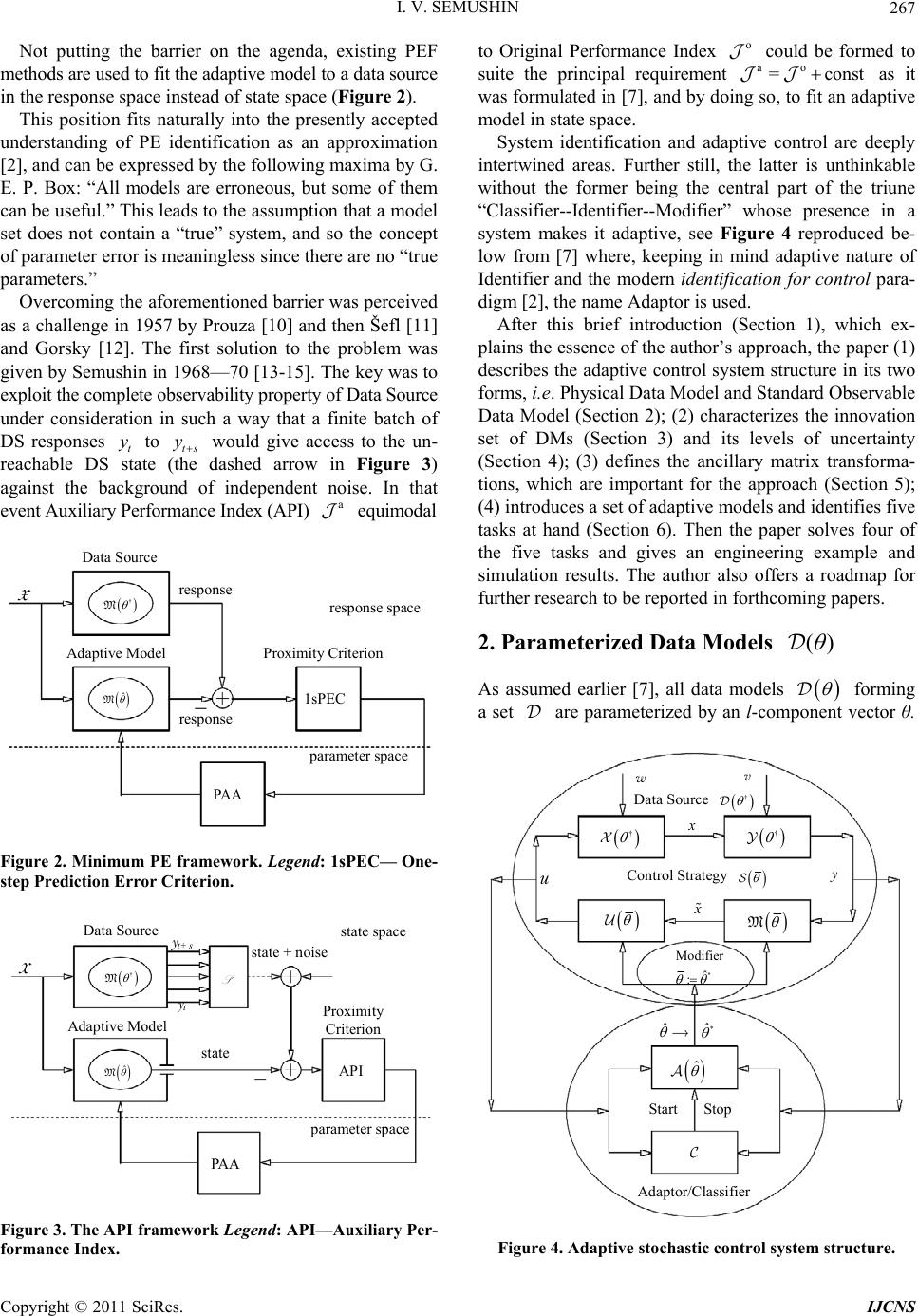 I. V. SEMUSHIN Copyright © 2011 SciRes. IJCNS 267 Not putting the barrier on the agenda, existing PEF methods are used to fit the adaptive model to a data source in the response space instead of state space (Figure 2). This position fits naturally into the presently accepted understanding of PE identification as an approximation [2], and can be expressed by the following maxima by G. E. P. Box: “All models are erroneous, but some of them can be useful.” This leads to the assumption that a model set does not contain a “true” system, and so the concept of parameter error is meaningless since there are no “true parameters.” Overcoming the aforementioned barrier was perceived as a challenge in 1957 by Prouza [10] and then Šefl [11] and Gorsky [12]. The first solution to the problem was given by Semushin in 1968—70 [13-15]. The key was to exploit the complete observability property of Data Source under consideration in such a way that a finite batch of DS responses t to ts would give access to the un- reachable DS state (the dashed arrow in Figure 3) against the background of independent noise. In that event Auxiliary Performance Index (API) a equimodal Data Source response 1sPEC response space Proximity Criterion response arameter space PAA X Adap tive Model † M ˆ M Figure 2. Minimum PE framework. Legend: 1sPEC— One- step Prediction Error Criterion. Data Source t AP I state space Proximi ty Criterion state arameter space PAA X Adaptive Model † M ˆ M t+ s state + noise S Figure 3. The API framework Legend: API—Auxiliary Per- formance Index. to Original Performance Index o could be formed to suite the principal requirement ao =const as it was formulated in [7], and by doing so, to fit an adaptiv e model in state space. System identification and adaptive control are deeply intertwined areas. Further still, the latter is unthinkable without the former being the central part of the triune “Classifier--Identifier--Modifier” whose presence in a system makes it adaptive, see Figure 4 reproduced be- low from [7] where, keeping in mind adaptive nature of Identifier and the modern identification for control para- digm [2], the name Adaptor is used. After this brief introduction (Section 1), which ex- plains the essence of the author’s approach, the paper (1) describes the adaptive control system structure in its two forms, i.e. Physical Data Model and Standard Observab le Data Model (Section 2); (2) characterizes the innovation set of DMs (Section 3) and its levels of uncertainty (Section 4); (3) defines the ancillary matrix transforma- tions, which are important for the approach (Section 5); (4) introduces a set of adap tive models and identifies five tasks at hand (Section 6). Then the paper solves four of the five tasks and gives an engineering example and simulation results. The author also offers a roadmap for further research to be reported in forthcoming papers. 2. Parameterized Data Models () As assumed earlier [7], all data models forming a set are parameterized by an l-component vector θ. † † M ˆ Start Stop * ˆ ˆ u Control Strategy w v Data Source † * Modifier ˆ : Adaptor/Classifier Figure 4. Adaptive stochastic control system structure. 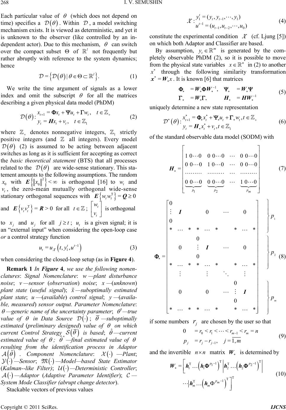 I. V. SEMUSHIN Copyright © 2011 SciRes. IJCNS 268 Each particular value of (which does not depend on time) specifies a . Within , a model switching mechanism exists. It is viewed as deterministic, and yet it is unknown to the observer (like controlled by an in- dependent actor). Due to this mechanism, can switch over the compact subset of l not frequently but rather abruptly with reference to the system dynamics; hence =| . l (1) We write the time argument of signals as a lower index and omit the subscript for all the matrices describing a given physical data model (PhD M) 1 1 =, :=, tttt ttt xxuwt yxvt H (2) where denotes nonnegative integers, 1 strictly positive integers (and all integers). Every model (2) is assumed to be acting between adjacent switches as long as it is sufficient for accepting as correct the basic theoretical statement (BTS) that all processes related to the are wide-sense stationary. This sta- tement am ounts t o t he following assumptions. The random 0 with 2 0<xE is orthogonal [16] to t w and t v, the zero-mean mutually orthogonal wide-sense stationary orthogonal sequences with T=0 tt ww EQ and T=>0 tt vvER for all t ; t t w v is orthogonal to and u for all jt; t u is a given signal; it is an “external input” when considering the open-loop case or a control strategy function 1 1 =,, tt t uutyu X (3) when considering the closed-loop setup (as in Figure 4). Remark 1 In Figure 4, we use the following nomen- clatures: Signal Nomenclature: w—plant disturbance noise; v—sensor (observation) noise; —(unknown) plant state (useful signal); —suboptimally estimated plant state; u—(available) control signal; y—(availa- ble, measured) sensor output. Parameter Nomenclature: —generic name of the uncertainty parameter; † —true value of in Data Source ; —suboptimally estimated (preliminary designed) value of on which current Control Strategy is based; ˆ —current estimated value of ; —final estimated value of resulting from the identification process in Adaptor ˆ . Component Nomenclature: —Plant; —Sensor; M—Model—based State Estimator (Kalman--like Filter); —Deterministic Controller; —Adaptor (Adaptive Parameter Identifier); — System Mode Classifier (abrupt change detector). Stackable vectors of previous values 111 112 0 =( ,,,) :=(,,, ) t tt t tt yyy y uuu u X (4) constitute the experimental condition X (cf. Ljung [5]) on which both Adaptor and Classifier are based. By assumption, m t y is generated by the com- pletely observable PhDM (2), so it is possible to move from the physical state variables n x in (2) to another through the following similarity transformation = xW. It is known [6] that matrices 1 1 =,= =, = WW W WHHW (5) uniquely determine a new state representation 1 1 =, :=, tttt ttt xxuwt yxvt H (6) of the standard observable data model (SODM) with 12 1 000 000 00 0 001 000 00 = 0 000 001 00 pp p m H (7) 1 2 0 00 0 ****** 0 00 =0 ****** 0 00 0 ****** m p p p I I I (8) if some numbers r are chosen by the user so that 01 1 1 0=<<< <= =,=1, mm jjj rrrr n prrjm (9) and the invertible nn matrix W is determined by TT 11 TT 12 11 22 T T 1 T = pp pm mm Wh hhh hh (10)  I. V. SEMUSHIN Copyright © 2011 SciRes. IJCNS 269 Numbers 12 ,,, m pp p are known as the partial observability indices, and so W will be called the ob- servability matrix. Benefits of this transformation will be seen later (at the end of Section 5). Remark 2 Since the eigenvalues of (2) remain unchanged in (6), the transformation (5) does not alter the dynamics of Data Source; it also has no effect on its inputs and outputs and so can be made at will. 3. Parameterized Innovations The above data model of a time-invariant data source will be referred to as the conventional model, no matter whether it is PhDM (2) or SODM (6)-(8). Another commonly used representation is the time-invariant (due to BTS) innovation model 11 1 11 = := t t ttttt ttt tt xxu yx M G H (11) with 1 t, the initial 00 10 = xu , and 00 =xEx, which is the well-known steady-state Kalman filter with the innovation process 1tt , the optimal state predictor 1tt , the gain 1 TT = HHH R , = GK, and satisfying the algebraic Riccati equation (ARE) [17] 1 TT TT =. HHH RHQ (12) Concurrently, another form 1 1 11 1 11 =, := , =, t tt tt tt tttt ttt tt xxut xx t yx t M K H (13) with the initial 0 00 = x, which is equivalent to (11), can be used wh ere tt is the optimal “filtered” estimator for t based on experimental condition X (4). When ranges (or switches) over as in (1), we obtain the set of Kalman filters =. l MM (14) Theorem 1 (Steady-state Kalman filter uniqueness [18]). Assume that in wide-sense stationary circumstances the following conditions hold: 1) is positive definite 0R; 2) Matrix pair , is detectable; 3) Matrix pair 12 T ,Q is stabilizable. Then the following assertions are true: a) Every solution 1tt to the matrix discrete-time Riccati equation TT 1 TT 11 1 1 1 1 =, = , tt tt tt tttttt tt t t PP Q PP PHHPH RHP (15) with the initial condition 00 0P has the limit 1= lim tt t PP (16) and this limit coincides with |1 |1 =lim T tttttt t Ex xx x ΣP which is the unique non-negative definite solution to ARE (12) and defines the covariance of one-step prediction error |1 |1ttt tt xx (17) in the Wiener-Kolmogorov filter (as t). b) The Kalman gain 1 TT |1 |1 = ttt tt PHHPH R (18) in the Kalman filter (KF) 1| | ||1|1 |1 |1 = = = tt ttt ttttt tt tt t tt xu xx yx K H (19) has the limit 1 TT == lim t t KHHHR (20) such that the estimate transition matrix = IKH (21) for M (13) is a stable limit. c) Weighting function WK tk h of the Wiener-Kolmo- gorov filter operating as the l.s. optimal one-step predictor 1WK WK |1 ==1 == t tttk kktk kk hy hy coincides (asymptotically as t and uniformly in k) with the weighting function KF 1 =k k hΦAK of the Kalman filter-predictor (15)-(21) computing KF 1 |1 =1 =1 == k ttktkt k kk hy y AK Remark 3 Theorem 1 is well-known, however this formulation is close to that given and completely proved in Fomin [18]. The basic notions used here (detectability, stabilizability and others) are known from literature, for example Wohnam [19]. Derivation of Kalman filter equa- tions (15)-(21) can be found in Maybeck [20] or Anderson 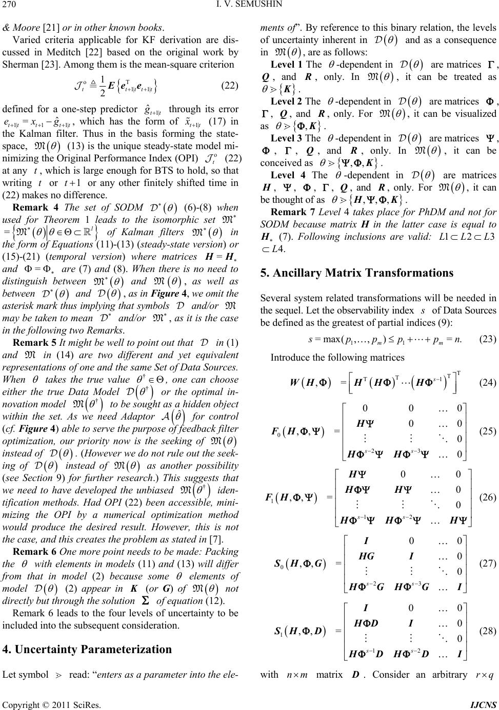 I. V. SEMUSHIN Copyright © 2011 SciRes. IJCNS 270 & Moore [21] or in other known books. Varied criteria applicable for KF derivation are dis- cussed in Meditch [22] based on the original work by Sherman [23]. Among them is the mean-square criterion oT1| 1| 1 2 ttttt Ee e (22) defined for a one-step predictor 1| ˆtt through its error 1|1 1| ˆ = tt ttt exg , which has the form of 1|tt (17) in the Kalman filter. Thus in the basis forming the state- space, M (13) is the unique steady-state model mi- nimizing th e Original Performan ce Index (OPI) o t (22) at any t, which is large enough for BTS to hold, so that writing t or 1t or any other finitely shifted time in (22) makes no difference. Remark 4 The set of SODM (6)-(8) when used for Theorem 1 leads to the isomorphic set M =l M of Kalman filters M in the form of Equations (11)-(13) (steady-state version) or (15)-(21) (temporal version) where matrices = H and = are (7) and (8 ). When there is no need to distinguish between M and M , as well as between and , as in Figure 4, we omit the asterisk mark thus implying that symbols and/or M may be taken to mean and/or M, as it is the case in the following two Remarks. Remark 5 It might be well to point out that in (1) and M in (14) are two different and yet equivalent representations of one and the same Set of Data Sources. When takes the true value † , one can choose either the true Data Model † or the optimal in- novation model † M to be sought as a hidden object within the set. As we need Adaptor ˆ for control (cf. Figure 4) able to serve the purpose of feedback filter optimization, our priority now is the seeking of M instead of . (However we do not rule out the seek- ing of instead of M as another possibility (see Section 9) for further research.) This suggests that we need to have developed the unbiased † M iden- tification methods. Had OPI (22) been accessible, mini- mizing the OPI by a numerical optimization method would produce the desired result. However, this is not the case, and this creates the problem as stated in [7]. Remark 6 One more point needs to be made: Packing the with elements in models (11) and (13) will differ from that in model (2) because some elements of model (2) appear in (or G) of M not directly but through the solution of equation (12). Remark 6 leads to the four levels of uncertainty to be included into the subsequent consideration. 4. Uncertainty Parameterization Let symbol read: “enters as a parameter into the ele- ments of”. By reference to this binary relation, the levels of uncertainty inherent in and as a consequence in M, are as follows: Level 1 The -dependent in are matrices , Q, and , only. In M, it can be treated as . Level 2 The -dependent in are matrices , , Q, and , only. For M, it can be visualized as , . Level 3 The -dependent in are matrices , , , Q, and , only. In M, it can be conceived as ,, . Level 4 The -dependent in are matrices , , , , Q, and , only. For M, it can be thought of as ,,, K . Remark 7 Level 4 takes place for PhDM and not for SODM because matrix H in the latter case is equal to (7). Following inclusions are valid: 123LL L 4.L 5. Ancillary Matrix Transformations Several system related transformations will be needed in the sequel. Let the observability index of Data Sources be defined as the greatest of partial indices (9): 11 =max(,,)= . mm ppp pn (23) Introduce the following matrices T T T T1 ,= s WHHHH (24) 0 23 00 0 00 ,, =0 0 ss H FH HH (25) 1 12 00 0 ,, =0 ss H HH FH HH H (26) 0 23 00 0 ,, =0 ss I HG I SH G GH GI (27) 1 12 00 0 ,, =0 ss I HD I SH D DH DI (28) with nm matrix D. Consider an arbitrary rq 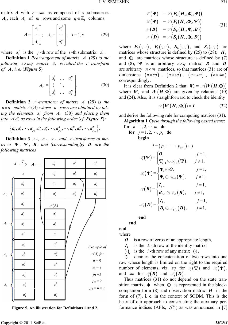 I. V. SEMUSHIN Copyright © 2011 SciRes. IJCNS 271 matrix A with =rsm as composed of submatrices i , each i of m rows and some 1 q columns: 1 1 =;=;=1, i i m si a is a A AA A (29) where i a is the j-th row o f the i-th submatrix i . Definition 1 Rearrangement of matrix (29) to the following mq matrix T is called the T-transform of , i. e. (Figure 5) 1 11 1 =. m T m ss aa aa A (30) Definition 2 S -transform of matrix (29) is the nq matrix S (A) whose n rows are obtained by tak- ing the elements i a from T (30) and placing them into S (A) as rows in the following order (cf. Figure 5): 1112 22 121 212 12 ,,,,,,,,, , ,,. mm m pp p m aaaa aaaaa Definition 3 F -, B -, P -, and N -transforms of ma- trices , , B, and (correspondingly) D are the following matrices 1 2 3 4 T T 1 1 a 2 1 a 3 1 a 1 2 a 2 2 a 3 2 a 1 3 a 2 3 a 3 3 a 1 4 a 2 4 a 3 4 a 1 1 a 1 2 a 1 3 a 2 1 a 2 2 a 3 1 a 3 2 a 3 3 a 3 4 a 1 1 a2 1 a 3 1 a 3 2 a 2 2 a 1 2 a 1 3 a 1 4 a2 4 a 2 3 a3 3 a 3 4 a (A) Example of S (A) for n = 9 m = 3 p1 =3 p2 = 2 p3 = 4 = s Figure 5. An illustration for Definitions 1 and 2. 0 1 0 1 =,, =,, =,, =,, FH FH BSHB DSHD FS BS PS NS (31) where 0,, F, 1,, F, 0,,S, and 1,, S are matrices whose structure is defined by (25) to (28); and are matrices whose structure is defined by (7) and (8); is an arbitrary nq matrix; B and D are arbitrary nm matrices, so that matrices (31) are of dimensions nsq, nsq, nsm, nsm correspondingly. It is clear from Definition 2 that =, WWH S where W and ,WH are given by relations (10) and (24). Also, it is straightforward to check the identity ** ,WH IS (32) and derive the following rule for computing m atrices (31). Algorithm 1 Cycle through the following nested items: for =1,2, ,km do for =1,2,, k p do begin 11 11 1 11 = , =1, =, 1, , =1, =, 1, , =1, =, 1, k i ii i i ii k i ii ippj j j j j j j O O I BBB F F B B P P 1 , =1, =, 1, k i ii j j I DDD N N end end end where O is a row of zeros of an appropriate length, k I is the k-th row of the identity matrix, i is the i-th row of any matrix (), denotes the concatenation of two rows into one row whose length is limited on the right to the required number of elements, viz. q for iF and i B, and m for iBP and iDN. Thus matrices (31) do not depend on the state tran- sition matrix when is represented in the block- companion form (8) and observation matrix in the form of (7), i. e. in the context of SODM. This is the heart of our approach to constructing the auxiliary per- formance indices (APIs, a t ) as was announced in [7]  I. V. SEMUSHIN Copyright © 2011 SciRes. IJCNS 272 and is considered below. Remark 8 The above matrix transformations as stated here were first introduced and used in [24]. 6. The Set of Adaptive Models ˆ M Let us define the set of adaptive models ˆˆ =l M (33) By this notation, we emphasize the fact that we construct adaptive models in the same class as M belongs to with the only difference that the unknown parameter in M is replaced by ˆ to obtain ˆ M. In so doing, each particular value of ˆ , an estimate of , leads to a fixed model ˆ M. In accordance with The Active Principle of Adaptation (APA) [7], only when ˆ ranges over in search of † for the goal † M or † M as governed by a smart, unsupervised helmsman equipped by a vision of the goal in state space (cf. Figure 3) and able to pursue it, we obtain an ada- ptive model ˆ M of active type within the set (33). In this case, ˆ will act as a self-tuned model parameter and so should be labeled by , the time ins- tant of model’s inner clock, in order to get thereby the emphasized notations ˆ and ˆ M in describing parameter adaptation algorithms (PAAs) to be developed. From this point on ˆ M becomes an adaptive estimator. Remark 9 Note in passing that pace of may differ from that of t: e.g. =kt for >0k. In general, there exist three time scales in adaptive systems, as stated by Anderson [3]: time scale for underlying plant dynamics, time scale for identifying plant, and time scale of plant parameters variation. We shall need discriminate be- tween and t later when developing a PAA. Remark 10 If we work in the context of SODM, the set ˆˆ =l M (34) instead of (33) should be used. At this junction, we identify the following tasks as pending: 1) Express ˆ M or ˆ M in explicit form. 2) Build up APIs that could offe r vision of the goal. 3) Examine APIs’ capacity to visualize the goal. 4) Put forward feasible schemata for APIs compu- tation. 5) Develop a PAA that could help pursueing the goal. Consider here the first four points consecutively. 6.1. Parameterized Adaptive Models Reasoning from (11), (13), we set the adaptive model 1| |1|1 |1 |1 ˆˆ = ˆ:ˆ = ttttt tt ttttt ggu yg MAFB C (35) or equivalently (due to =BAD) the model 1| | ||1 |1 |1 |1 ˆˆ = ˆˆ := ˆ = tttt t tt tttt ttttt ggu gg yg M AF D C (36) as a member of (33). Here ˆ,,,, ABC DF is the self-tuned parameter intended to estimate (in one-to- one correspondence) parameter ,, ,, GHK. In parallel, reasoning from M (cf. Remark 4), we build the adaptive model 1| |1|1 |1 |1 ˆˆ = ˆ:ˆ = ttttt tt ttttt ggu yg MAFB H (37) or equivalently (due to =BAD) the model 1| | ||1 |1 |1 |1 ˆˆ = ˆˆˆ := ˆ = tttt t tt tttt ttttt ggu gg yg M AF D H (38) with and = A taken in the form of (7) and (8). Adaptor ˆ using (35)-(36) (or alternatively, ˆ using (37)-(38)) is supposed to contain a PAA to offer the prospect of convergence. As viewed in Fig- ures 1 to 3, convergence can take place in three spaces: in response space; this is model response conver- gence, in state space; this is model state convergence, and in parameter space; this is model parameter con- vergence. For convergence of the last-named type, we anticipate almost surely (a.s.) convergence, as it is the case for MPE identification methods [16]. It actuates either or both of the two other types of convergence. The type of convergence in state space, as well as in response space, is induced by the type of Proximity Criterion, PC (cf. Figures 1-3). As seen from (22), we are oriented to the PC, which is quadratic in error; this being so, it would appear reasonable that these covergences would be in mean square (m.s.). Thus we anticipate the following properties of our estimators: a.s. † m.s. †m.s. 1| 1| m.s. †m. s. || ˆ ˆˆ : ˆˆ tt tt tt tt t gx gx MM MM (39) With the understanding that errors for PC 1|1 1||| 1|1|1|||| ˆˆ , ˆˆ , tt ttttt ttt tttt tt tttt tt exgexg rxgrxg (40)  I. V. SEMUSHIN Copyright © 2011 SciRes. IJCNS 273 are fundamentally unmeasurable, we search for a function | 11| ˆˆ ()= ts tstn tttt fy y (41) of the difference in two terms: outputs 1 ts t generated by Data Source described in any appropriate form (2), (6), (11), or (13), an d their estimates | 1| ˆtst tt y generated by the adaptive model ˆ M (or ˆ M). For ˆ t in (41), we will also use notations 1|tt or |tt , thus bring- ing them into correlation with 1|tt e or |tt e (corre- spondingly, with 1|tt r or |tt r) from (40). Then T aa 1 ˆˆˆ =2 ttt t E (42) will be taken as the PC and determined with the key aim: True (Unbiased) System Identifiability Here, the equivalence symbol needs clarification. Its sense correlates with the above concept of conver- gence (39). Necessary refinements will be done (in Theorem 2). 6.2. API Generalized Residual Since (41) requires many-step-predicted value | 1| ˆtst tt y as a stackable vector T |TT T 1|1|2|| ˆˆˆ ˆ =||| tst tttttttst yyy y (43) we supplement our model (35), (36) with the k-step ahead predictors |1|1 || ˆˆ ==1, ˆˆ = tkttk ttk tkt tkt ggu ks yg AF C (44) and call the residual in (41) by Generalized Residual || 1|11| ˆ GR := tstts tst ttt tt yy (45) Recursively using (2) with no tations (2 3) -(2 8) yields 1101 011 1 11 1 11 =, ,, ,, =, ,, ,, ts ts tt t tsts tt ts ts ttt ts ts tt yx u wv yxu wv WHF H FH WH FH FH ΦΦΨ Ψ (46) From (11)--(13) by the same technique, we obtain 11|01 |1 01| 1 1|1 |1 01| =, ,, ,, =, ,, ,, ts ts tttt tsts tt ts ts tttt tsts tt yx u yxu WHF H SH G WH FH SH G (47) Applying the same technique to (35), (36) together with (44) yields | 1|1| 01 |1 1|| 1 ˆˆ =, ,, ˆˆ =, ,, tst ts tt ttt tst ts tttt t yg u ygu WCAFCAF WCAA FCAF (48) and ||1 11|01| ˆ =,, ts tsttsts ttt tt yy SCAB (49) Remark 11 The following diagram (Figure 6) shows that so far we have obtained formulae (46) to (49) only for the PhDM. We now turn to the case of SODM (by application of (5)). In this case, substituting from (7) for and C into (46)-(48) as well as taking there = and = A in the form of (8) and using transformations (31), we obtain: a) for the conventio nal form — 11 1 11 1 1 11 = = ts ts tt t tsts tt ts ts ttt ts ts tt yx u wv yxu wv Ψ Ψ SF FS SB BS (50) b) for the innovation form — PhDM SODM (6)-(8) (2) (46) (50) (11)-(13)(35)-(36) (11)-(13) (35)-(36) (51) (52) (53) (49) (48) (47) C = Conventional form I = Innovation form M C M ˆ M * M *ˆ M (5) * Figure 6. Taxonomy of models. The arrows indicate the consequtive order in which the numbered formulae are obtained.  I. V. SEMUSHIN Copyright © 2011 SciRes. IJCNS 274 11| 1 |1 1| 1 1| |1 1| = = ts ts ttt t tsts tt ts ts tttt tsts tt yxu yx u G G SF P SB P (51) c) for the predicted values — | 1| 1|1 |1 1| | ˆˆ = ˆˆ = tst ts tt ttt tst ts tt ttt yg u ygu SF SB F AF (52) and using S-transform in (49) yields ||1 11| 1| ˆ = ts tsttsts ttt tt yy BSS P (53) Now that we have written formulae (46) to (53), many of them arranged in pairs, we find all possible representa- tions for the GR by substituting these equations into (45): 1) for the PhDM with the predicted output 1| ˆtt — the 1st of (46) minus the 1st of (48) ives (54) | 1|1 1| 001 011 ˆ =, , ,, ,, ,, tst ttt tt ts t tsts tt xg u wv WH WCA FH FCAF FH (54) the 1st of (47) minus the 1st of (48) ives (55) | 1|1| 1| 001 |1 01| ˆ =, , ,, ,, ,, tst tttt tt ts t tsts tt xg u WH WCA FH FCAF SH (55) 2) for the PhDM with the filtered output | ˆtt — the 2nd of (46) minus the 2nd of (48) ives (56) | 1| | 1 11 1 11 ˆ =, , ,, ,, ,, tst ttt tt ts t ts ts tt xg u wv WH WCAA FH FCAF FH (56) the 2nd of (47) minus the 2nd of (48) ives (57) | 1| | 1 11 |1 01| ˆ =, , ,, ,, ,, tst ttt tt ts t tsts tt xg u WH WCAA FH FCAF SH G (57) and from (49) (taking into accoun t (27)-(28) and relation =BAD), we have ||1 1|01| |1 11| =,, =,, tsttsts tt tt tsts tt SCAB SCAD (58) 3) for the SODM with the predicted output 1| ˆtt — the 1st of (50) minus the 1st of (52) ives (59) | 1|11| 1 11 = tst ttt tt ts t ts ts tt xg u wv F S FF FS (59) the 1st of (51) minus the 1st of (52) ives (60) | 1|1|1| 1 |1 1| ˆ = tst tttt tt ts t tsts tt xg u ΨF G S FF P (60) 4) for the SODM with the filtered output | ˆtt — the 2nd of (50) minus the 2nd of (52) ives (61) | 1| | 1 11 ˆ = tst ttttt ts t ts ts tt xg u wv A F S BB BS (61) the 2nd of (51) minus the 2 nd of (52) ives (62) | 1|| | 1 |1 1| ˆ = tst t ttttt ts t tsts tt xg u A F G S BB P (62) and from (58) (taking into account (31)), we have ||1|1 1| 1|1| == tst tstststs tt tttt BDSPN (63) Generalized Residual, as introduced in (45), is impor- tant in allowing the user to extract all possible amount of information from experimental condition X (4) con- cerning the unmeasurable errors (40). The foregoing equa- tions (54) to (63) reveal the features of GR from the practical standpoint as a possible tool for system identifi- cation under different levels of uncertainty and with dif- ferent data models used: PhDM or SODM. 6.3. API Identifiability of † M Let the auxiliary process (41) for the API (42) be built as 1|1 1|1 |1 1| ˆ = = ts ts ttt ttt tsts tt yg u F B SF P (64) (Figures 7 and 8) or, equivalently, as 1 |1| |1 1| ˆ = = ts ts ttt ttt tsts tt yg u AF D S B N (65) (Figures 9 and 10). Theorem 2 Let ˆ t (41) be a vector-valued n- component function of (45). If ˆ t is defined by (64) or (equivalently) (65) in order to form the API (42), then minimum in ˆ of the API fixed out at any instant t is  I. V. SEMUSHIN Copyright © 2011 SciRes. IJCNS 275 ts y * t y t u D * min ,, DF a t T T 1tt ts u ts y * Figure 7. Adaptor based on 1|tt , the first equality in (64). denotes the unitary delay operator. 1tt * G min ,, DF a t P 1tt ts u ts * H 1tsts Figure 8. Adaptor based on 1|tt , the second equality in (64). 1tt A B * G min ,, BF a t B tt 1ts u ts y * H S t u t y 1 ˆtt Figure 9. Adaptor based on |tt , the first equality in (65). 1tsts F A * min ,, DF a t N tt ts u * H 1 ˆtsts K ts y 1tt Figure 10. Adaptor based on |tt , the second equality in (65). the necessary and sufficient condition for adaptive model ˆ M to be consistent estimator of † M in mean square, m.s. † ˆ :t MM, that is True (Unbiased) m.s. System Identifiability 2 a1| 1| ˆˆˆ=0 min ttt tt xg ⇔E in the following three setups: Setup 1 (Random Control Input) ut is a preas- signed zero-mean orthogonal wide-sence stationary pro- cess orthogonal to ,wtvt but in contras t to {()}wt and vt , known and serving as a testing signal; Setup 2 (Pure Filtering) :=0tut , and Setup 3 (Close-loop Control) with known = . Proof: See the Appendix. Corollary 1 Under the assumptions of Theorem 2, mi- nimum in ˆ of the API fixed out at any t is the necessary and sufficient condition for adaptive model ˆ M to be consistent estimator of † M in mean square, m.s. † ˆ :t MM, up to the equality 1|11|1 ˆ = ts ts ttt ttt ugu FFF (66) or, what is equivalent, equality 11 || ˆ = ts ts tttttt xugu BBAF (67) Corollary 2 Under the assumptions of Theorem 2, if upper rows of and are zero, then in Corollary 1 equalities (66)-(67) are replaced by equalities 1| 1||| ˆˆ := ;= jii tt tttttt txgxg A (68) where =1, 1js and =1,is are numbers of vector components. If additionally 0 t u or if {} t u is ortho- gonal to {} t w and {} t v for models (11), (13), (35) and (36), then equalities (68) hold for all vector components, and the following equalities =, =,=,=ABGDKF (69) are added to (68) thus assuring that m.s. † ˆ MM. Proof of (68 ) and = leans upon Algorith m 1 for computing matrix F (see Section 5). After that, equali- ties = , = G and =DK follow from unique- ness of Kalman filter equations. Corollary 3 If , , Q, and are unknown and (7) and known, thereby allowing for situation when ˆ, A,B D, then in Corollary 1 equalities (66)- (67) are replaced by equalities 1|1|| | ˆˆ :=,= =, =, = tt tt tt tt txgxg BG DK (70) thus assuring that m.s. † ˆ MM .  I. V. SEMUSHIN Copyright © 2011 SciRes. IJCNS 276 6.4. API Identifiability of † M When transformation of PhDM, M to SODM, M is troublesome or objectionable, we have to work with the given PhDM. In this case, we take, as ˆ t for (42), either of the two processes: |1| 1|11||11 1| =;=, tsttst tttt tttt WW (71) where relation (58) can be used. In (71), we denote: 1 to be an (nn)-matrix; 1 an ()mn-matrix, and 111 =,WWH with ,W defined by (24). We assign matrices 1 , 1 rather arbitrarily choosing them as substitutes for unknown matrices and from the conditions: 10 and 1= rn ank W. By the latter condition, the pseudo-inverse matrix 1 W is found as 1 TT 111 WWW, and the following ()nn-matrices 11 11 01 0 ˆ ,; , ˆˆ ; TWWH TWWCA TT TTA (72) are non-singular if the addional conditions 0;rank ,= 0;rank ,= n n WH AWCA (73) hold. The last-added term in (55), as well as in (57), does not depend on the model parameter ˆ, A,B,C, DF and is formed by the innovation process 1|tt , which is an orthogonal process. In addition, the set M of models (35), or equivalently (36) contains the optimal model (11), (13). On this grou n ds , we c ome to the following result. Theorem 3 Let ˆ t (41) be a vector-valued n- component function of (45). If ˆ t is taken from (71) in order to form the API (42), then minimum in ˆ, A,B,C, DF of the API fixed out at any instant t is the necessary and sufficient condition for adaptive model ˆ M to be consistent estimator of † M in mean square, m.s. † ˆ :t MM up to the equations 1| 1| 10 01 ˆˆ =,,,, tt tt ts t xg u T WFCAF FH (74) in case of the first process of (71), and 0|0 | 11 11 11 ˆˆ =,,,, tt tt ts t xg u TT WFCAF FH (75) in case of the second process of (71) taken to form the API. Proof: Given in [25]. Corollary 4 On the assumption that , Q and are unknown, but , and known, i. e. allowing for situation when ˆ, BD and 1= H, 1= in (71), equalities (74) and (75) in Theorem 3 are replaced by equalities 1|1| | | ˆˆ :=;= =, = tt tt tt tt txgxg BG DK (76) This follows from the right sides of (74)-(75) being zero and from 00 ˆˆ == ==TTT TI under the assumption of this corollary. Remark 12 The similar result however relating to the second process of (71) only and in the following form of Learning Criterion (LC) 1T 1|1|1|1 : ˆ=0 ts ttttttt t yg EW WD with =,WWH , and matrix D being the only adjustable parameter of filter (36) in the event that = , CH, and 0 t u , was also obtained [26] and restated in a different way [27] by Hampton where the problem of minimizing LC in the form of 2 11|1|1 ˆ ts ttttt yg WW D was formulated. The convergence properties of Hamp- ton’s solution were studied by Perriot-Mathonna [28]. Corollary 5 On the assumption that , , Q and are unknown and 0 t u , i. e. allowing for situation when ˆ A,B,C,D, equalities (74) and (75) in Theorem 3 are replaced by equalities 1|1| || 11 ˆˆ :=;= =;=;=;= t tt ttttt tgxgx G SS SSBSCHSDSK (77) where is an arbitrary non-singular ()nn-matrix. The proof is obtained by setting the right sides of (74)-(75) to zero if definitions (72) are accounted for. In so doing, we consider 1 ˆ = TT (or 1 0 ˆ = TT) an unknown matrix of similarity transformation. A pure algebraic proof of the result is also available due to [25,29]. Analyzing conditions of Corollary 5 in more detail, state the following results. Corollary 6 On the assumption that , , Q and are unknown and known and 0 t u, i. e. allow- ing for situation when ˆ , A,B D and CH, equalities (74)-(75) in Theorem 3 are replaced by equa- lities 1|1| || 1 ˆˆ :=;= =;=;= t tt ttttt tgxgx S ASSBSGDSK (78) where is a non-singular ()nn-matrix subject to relation = HS . Corollary 7 On the assumption that , Q, and are unknown and known and 0 t u, i. e. allow- ing for situation when ˆ B,C,D and = , equa- lities (74)-( 75) in Theorem 3 are replaced by equalities  I. V. SEMUSHIN Copyright © 2011 SciRes. IJCNS 277 1|1| || 1 ˆˆ :=;= =; =;= tt tttt tt tgxgx S BSGCHS DSK (79) where is a non-singular ()nn-matrix subject to relation = S. Corollary 8 On the assumption that , Q, and are unknown and known and 0 t u, i. e. allow- ing for situation when ˆ, BD, = and CH, equalities (74)-(75) in Theorem 3 are replaced by equa- lities 1|1|| | ˆˆ :=;= =, = tt tttt tt tgxgx BG DK (80) This is a special case of Corollary 4 at 0 t u. Corollary 9 If under the assumptions of Corollary 6 = rn ank H, then = I (cf. theorems of [30]). Corollary 10 If under the assumptions of Corollary 6 matrix is given by (7) and is sought in the form of (8), then = W when W is matrix (10). If in ad- dition has the form of (8), then = I. This establishes the association of this case with the identifiability of matrices , G and for SODM — cf. Corollary 3. Corollary 11 For the adaptive model (35)-(36), which is optimal in structure, ()nn-matrix cannot be identified with the APIs under consideration, i. e. it must be known. As this takes place, the whole amount of identifiable entries of matrix is ()mn. This follows from Corollary 7 where we have the Fro- benius Problem of finding matrices commutative with the given matrix . It is known that the total number of linear independent solutions to the problem is not less than n. The second part of Corollary 11 is ob- tained from similarity (isomorphism) of any system (2) to its standard observable form (6)-(8). 6.5. Main Conceptual Novelty The goal of an identification method is to find a model, whose “behavior” best approximates that of the system under consideration. However, what meaning may be at- tributed to the term “behavior”? In the context of APA, the inner state of a dynamical system is emphasized, whereas classical MPE methods imply the output behavior. Theorems 2-3 and corollaries solve the task by an in- direct minimization of either the er rors (40) in prediction or mean square estimation of the inner state, whereas classical MPE methods do so by a direct minimization of a “prediction error criterion,” which expresses the one- step “prediction performance” of the model on the given input-output experimental condition (4). The difference is illustrated graphically in Figures 2 and 3. At the same time, both approaches share a common trait of having a proximity criterion to be numerically minimized. Sub- space-based identification methods [31] also put em- phasis on state of a dynamical system, but by doing the following: combining the past input-output data and fu- ture inputs linearly to predict future outputs; minimizing the error of prediction measured in the Frobenius norm; obtaining the KF state sequence by using the robust Singular Value Decomposition; and finally, estimating system matrices with Least Squares techniques. Theorem 2 and its corollaries establish the point that generally, the API approach is rather useful as it helps us identify unknown parameters of optimal discrete time filters used either independently or as a part of a control strategy. It also indicates the levels of uncertainty (see Section 4), within which the approach still remains practicable. General characteristic values of these levels are defined by three setups stated in the theorem (and realistically reproduced in Proof). Corollary 1 is an ac- curate generalization of Theorem 2 for the case where there is no point in specifying Setups 1, 2 or 3. A few details of the levels are stated by Corollaries 2 and 3. Feasible schemata for APIs computation visually support these identification results associated with the standard observable data model, SODM (Figures 7-10), and the physical data model, PhDM (see below Figures 11-14). K min D 1tt t u H 1 ˆtt y 1t y 1 ˆtt g H a t 2t y 3t y ts y H H 2 ˆtt y 3 ˆtt y ˆtst y 1t u 2t u W (1) 1ts u (2) (3) (3) (2) (1) Figure 11. Adaptor based on process 1|tt from (71) and relation (48) under assumptions of Corollary 4. Here ˆ D.  I. V. SEMUSHIN Copyright © 2011 SciRes. IJCNS 278 K min tt H 1 ˆ tsts H a t ts y H H 1tt 1ts u (2) (s) 1tsts (s-1) (2) (1) ( -1) ( ) W Figure 12. Adaptor based on process |tt from (71) and rela- tion (58) under assumptions of Corollary 4. Here ˆ D. G min tt 1 ˆtsts a t ts y 11 tt 1ts u (2) ( ) 1tsts (s-1) (2) ( -1) ( ) W Figure 13. Adaptor based on process 1|tt from (71) and rela- tion (58) under assumptions of Corollary 4. Here ˆ B. SK min , D 1tt H 1 ˆtt H a t H H 1 SS 1t (1) ( ) ( -1) (2) ( -1) ( ) 1 W (1) (2) ˆtt 2t y ts y Figure 14. Identification of and K as parameters of optimal steady-state filter. Here ˆ , AD and 0 t u . 6.6. API Adaptor Forms We have stated the uniqueness of identification under conditions of corollaries 2 to 4 and 8 to 10. This is expressed by equalities (69), (70), (76), and (80). Iden- tification is accomplished non-uniquely—up to arbitrary similarity transformation if conditions for corollaries 5 to 7 hold. This situation is expressed by equalities (77)-(79). Uniquely accomplished identification is possible in some particular cases, as stated in corollary 6 and shown in Figure 14. In this figure, PhDM is used where 1 W 11 =,WH . Matrices and are identifiable when is known and if equations = SH and = S imply = I where is a matrix differing from only in that unknown parameters are denoted differently (cf. Corollary 8). On this condition, .. 1| 1| ˆms tt tt x and .. || ˆms tttt x. When Figures 7-10 are compared with Figures 11-14, it is apparent that Adap tor for SODM is much simpler than Adaptor for PhDM. These benefits can be realized only if the transition from (2) to (6) has been preliminary per- formed. If it is the case, the estimates in terms of PhDM can be obtained according to the following statement.  I. V. SEMUSHIN Copyright © 2011 SciRes. IJCNS 279 Corollary 12 Let W (10) be defined analytically as a known function 0 = WW of the unknown para- meters 00 01 1 =,, N entering 0 = of (2) and to be identified by minimization of criterion (42), and 1 Nmn as stated by Corollary 11. Let matrix 1 = WW be found in the companion form (8) as a known function of 0 , namely = where vector 12 =,, N is composed of 2 N non- trivial ( i.e. non-zero ot non-unit) unknown entries of (12 0<NNmn), and in so doing the type of function 0 =f be determined as continuous function hav- ing its inversion 1 0=f (the last-named hypothesis can be true as 12 NN). Then minimization of (42) under conditions of Co- rollary 3 ensures , as necessary and sufficient condition, attaining the following limits: m.s. 11 1| 1| m.s. 11 || a.s. 111 a.s. 11 ˆ ˆ tt tt tt tt ag x ag x fa fa fa W W WAW WD K (81) where a are the adjustable parameters of matrix , taken in the form (8), if a.s. a by a PAA. Proof: Done by inverting equalities (78), see Corol- laries 6 and 10. Thus the corresponding block-diagram (Figure 15) dif- fers from the preceding block-diagram (Figure 14) by in- cluding the operations turning back from SODM to PhDM by relations (81). However, some questions remain open: “Must of necessity the transition from PhDM to SODM min , AD 1tt H 1 ˆtt a t t 1 S 2 ts A 0 1 ˆtt Figure 15. Using ˆ M (34) for D (2) with the pro- perty 1 ** AWW and * WK. Legend: 1—operation 1 *0 W; 2---operation 1 a . and back be performed? What benefits are harboured by the transition if not performed ?” 7. Engineering Illustration & a Rule Consider a simplified version of the application problem from aeronautical equipment engineering [32] whose com - plete statement is given in [33]. The simplified version is the instrument error model for one channel of the Inertial Navigation System (INS) of semi-analytical type, which looks as follows: 1 1 1 10 10 =000 0001 0 0 0 =1 000 x Ax Gy t x t Ax Gy t ttt vg a mb n v w ma n yxv (82) where s ubscr ipts , , A, and G stand for “axis Ox ”, “axis Oy”, “Accelerometer”, and “Gyro”, correspond- ingly.1 State vector T =,,, xAxGy vmn x consists of: v , random error in reading velocity along axis Ox of a gyro-stabled platform (GSP); , angular error in deter- mining the local vertical; Ax m, the accelerometer read- ing random error; and Gy n, the gyro constant drift rate. Parameters 2 11 1 11 =1 2aHb H and 111 =exp1b are obtained from the correla- tion function 2 11 =exp|| mAx RtH t (83) describing Ax m after transition from continuous time t in (83) to the discrete—time index t in (82) with the sampling period . Let parameters 1 and 1 be unknown. Rewriting (82) in terms of 1 = Ax Ax ma results in that parameters 1 a and 1 b move into of equations (2) with 1 1 100 100 =,= 00 01 0001 0 ga a b (84) and =1 000H. Using (10) in (5) gives (6) with *= H and 1These subscripts are a tribute to the engineering tradition: must not be confused with x denoting the state vector.  I. V. SEMUSHIN Copyright © 2011 SciRes. IJCNS 280 1 *11 2 111 2 * 4321 41 31 21 11 0 =1 1 = 0100 0010 =0001 =1 =3 1 =3 3 =3 a ba bba ga b b b b (85) As seen from (85), parameter 1 a vanishes in * . This is quite reasonable, because it belongs, by its nature, to of (82) (and * of (85)), that is 1 a has entered of (84) artificially. However it is very difficult to reveal the presence of such non-identifiable parameters in by visual appearance. Transition to SODM reveals such problem parameters, as it is the case for (85), and this is its benefit although this may prove to be a difficult algebra. The question, that ended Section 6.6, can be refor- mulated: “Is it always necessary to move from PhDM to SODM in order to reveal non-identifiable parameters in matrix ?” The answer is: “No,” and it is given by Co- rollary 6 (Section 6.4) from where we obtain the following General Rule: (Algebraic Identifability Criterion) 1) Take as it is up to the unknown para meters. 2) Take in the same form as , but using other designations for the unknown parameters. 3) Take an arbitrary nn matrix , det 0 sat- isfying equation = S (matrix must be known). 4) Write = S in the component-wise form. 5) If = I is the only solution, the unknown para- meters of are identifiable; you ne ed not do the transition to SODM. 6) If = I is not the only solution, find the constraints needed to have the solution = I as unique. 7) Those parameters that require to maintain the found constraints may be non-identifiable; they become identifiable only if the constrains are fulfilled. Following this Rule in the example yields 1 1 101 0 10 10 ,and 000 000 0001 0001 xx yy 21 222324 31 323334 41 424344 1000 sss sss sss S where the following known constants are non-zero: , , and ; the following entries are unknown: 0x , 10x , 1y , 11y ; and ||0S. Comparing left and right sides of = S (this is much more simpler than the transition to SDOM) yields the unique solution 1= y and 33 =[1,1,,1] diag sS where 33 1 = xx . Element y (that equals 1 b in (84)) is thus seen to be identifiable even if (that equals 1 a in (84)) is in error. However is not identifiable, that is it should be estimated by some other methods. Notice that in active type identification, there is no need to identify 1 = a because optimal gain and matrix are being esti- mated directly—avoiding estimation of , Q and (this is the general result). 8. Simulation Example E1 Second order system with unknown covariances Q and of the noises t w and t v is given by 112 01 00 = =10 tttt ttt xuw ff yxv =0.4 , =1.0 , 1=0.8f and 2=0.1f. Kalman gain T 12 =[ |]kkK should be estimated by adaptive model gain T 12 =[ |]ddD, 12 ˆ=( ,)dd . E2 The same system as in E1. Unknowns are Q, , and 12 , f of matrix . Adaptive model parameter is the four-componen t vector: 1212 ˆˆ ˆ=,,, fdd . We analyze the adaptive model behavior with the Integral Percent Error (IPE) defined by IPEOPT OPT ˆˆ ˆ =( )/100% (86) with respect to OPT ˆ , the optimal value of ˆ for dif- ferent levels of signal-to-noise ratio, =SNRQR. Results of Figures 16-17 are obtained in conext of Figure 10 using the simulation toolbox developed by Gorokhov [34]. The results of this and other simulation experiments confirm applicability of the presented me- thod. 9. Conclusions This paper develops The Active Principle of Adaptation for linear time-invariant state-space stochastic MIMO filter systems included into the feedback or considered 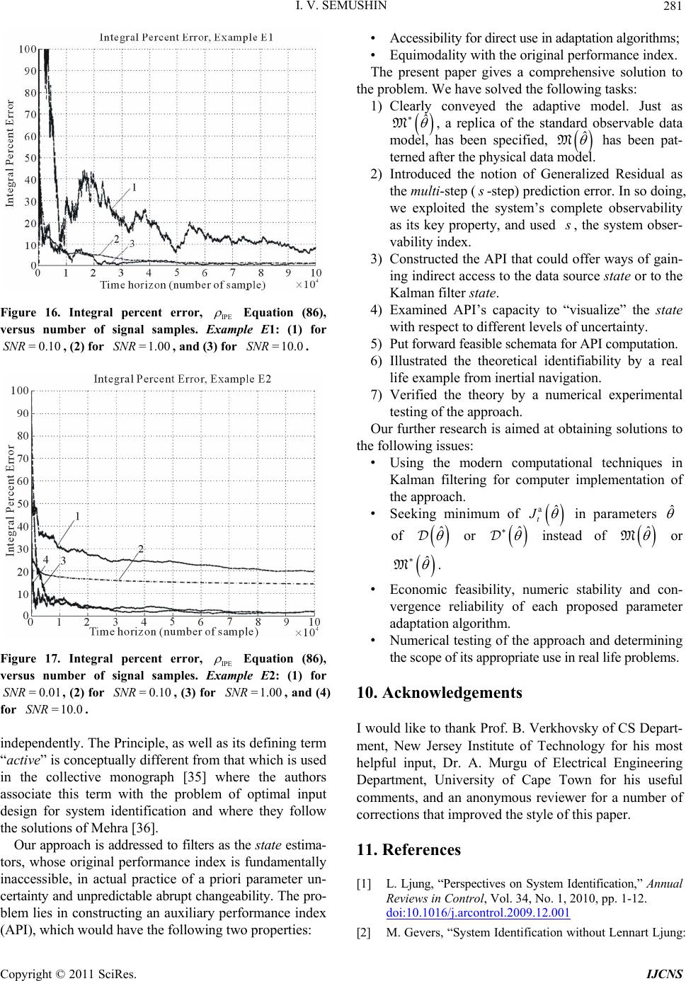 I. V. SEMUSHIN Copyright © 2011 SciRes. IJCNS 281 Figure 16. Integral percent error, IP E Equation (86), versus number of signal samples. Example E1: (1) for =0.10SNR , (2) for =1.00SNR, and (3) for =10.0SNR. Figure 17. Integral percent error, IP E Equation (86), versus number of signal samples. Example E2: (1) for =0.01SNR , (2) for =0.10SNR , (3) for =1.00SNR , and (4) for =10.0SNR . independently. The Principle, as well as its defining term “active” is conceptually different from that which is used in the collective monograph [35] where the authors associate this term with the problem of optimal input design for system identification and where they follow the solutions of Mehra [36]. Our approach is addressed to filters as the state estima- tors, whose original performance index is fundamentally inaccessible, in actual practice of a priori parameter un- certainty and unpredictable abrupt changeability. The pro- blem lies in constructing an auxiliary performance index (API), which would have the following two properties: • Accessibility for direct use in adaptation algorithms; • Equimodality with the original performance index. The present paper gives a comprehensive solution to the problem. We have solved the following tasks: 1) Clearly conveyed the adaptive model. Just as ˆ M, a replica of the standard observable data model, has been specified, ˆ M has been pat- terned after the physical data model. 2) Introduced the notion of Generalized Residual as the multi-step ( -step) prediction error. In so doing, we exploited the system’s complete observability as its key property, and used , the system obser- vability index. 3) Constructed the API that could offer ways of gain- ing indirect access to the data source state or to the Kalman filter state. 4) Examined API’s capacity to “visualize” the state with respect to different levels of uncertainty. 5) Put forward feasible schemata for API computation. 6) Illustrated the theoretical identifiability by a real life example from inertial navigation. 7) Verified the theory by a numerical experimental testing of the approach. Our further research is aimed at obtaining solutions to the following issues: • Using the modern computational techniques in Kalman filtering for computer implementation of the approach. • Seeking minimum of aˆ t J in parameters ˆ of ˆ or ˆ instead of ˆ M or ˆ M. • Economic feasibility, numeric stability and con- vergence reliability of each proposed parameter adaptation algorithm. • Numerical testing of the appro ach and determining the scope of its appropriate use in real life problems. 10. Acknowledgements I would lik e to thank Prof. B. Verkh ovsky of CS Depar t- ment, New Jersey Institute of Technology for his most helpful input, Dr. A. Murgu of Electrical Engineering Department, University of Cape Town for his useful comments, and an anonymous reviewer for a number of corrections that improved the style of this paper. 11. References [1] L. Ljung, “Perspectives on System Identification,” Annual Reviews in Control, Vol. 34, No. 1, 2010, pp. 1-12. doi:10.1016/j.arcontrol.2009.12.001 [2] M. Gevers, “System Identification without Lennart Ljung:  I. V. SEMUSHIN Copyright © 2011 SciRes. IJCNS 282 What Would Have Been Different?” In: T. Glad and G. Hendeby, Eds., Forever Ljung in System Identification, Studentlitteratur AB, Norrtalje, 2006. [3] B. D. O. Anderson, “Two Decades of Adaptive Control Pitfalls,” Proceedings of the 8th International Conference on Control, Automation, Robotics and Vision, Kunming, December 2004. [4] V. V. Terekhov and I. Y. Tyukin, “Adaptive Control Systems: Issues and Tendencies,” Control and Information Technology, St. Petersburg University of Information Tech- nology, St. Peters burg, 2 003, pp . 146-1 54. [5] L. Ljung, “Convergence Analysis of Parametric Identi- fication Methods,” IEEE Transactions on Automatic Con- trol, Vol. AC-23, No. 5, 1978, pp. 770-783. doi:10.1109/TAC.1978.1101840 [6] L. Ljung, “System Identification: Theory for the User,” Prentice-Hall, Inc., Englewood Cliffs, 1987. [7] I. V. Semushin, “Adaptation in Stochastic Dynamic Sys- tems—Survey and New Results I,” International Journal of Communications, Network and System Sciences, Vol . 4, No. 1, 2011, pp. 17- 23. doi:10.4236/ijcns.2011.41002 [8] R. K. Mehra, “Approaches to Adaptive Filtering,” IEEE Transactions on Automatic Control, Vol. AC-17, No. 5, 1972, pp. 693-69 8. doi:10.1109/TAC.1972.1100100 [9] R. E. Kalman, P. L. Falb and M. A. Arbib, “Topics in Mathematical System Theory,” McGraw Hill, Boston, 1969. [10] L. Prouza, “Bemerkung Zur Linearen Prediktoren Mittels Eines Lernenden Filters,” Transactions of the 1st Prague Conference on the Information Theory and Statistical Deci- sion Functions, Prague, 28-30 November 1956, pp. 37-41. [11] O. Šefl, “Filters and Predictors Which Adapt Their Values to Unknown Parameters of the Input Process,” Transactions of the 2nd Prague Conference on the Information Theory and Statistical Decision Functions, Prague, 1961, pp . 597-608 . [12] A. A. Gorsky, “Automatic Optimal Filtering,” Transactions on Power Engineering and Automation, USSR Academy of Sciences, Engineering Division, Moscow, No. 4, 1962, pp. 3-30. [13] I. V. Semushin, “Use of Active Principle for Filtering Non- stationary Random Processes,” Proceedings of the 3rd Sci- ence and Technology Conference—Novgorod LETI Branch, St. Petersburg, 19 68, p . 64. [14] I. V. Semushin, “Multi-Channel Adaptive Filter of Active Type,” Transactions on Instrument Making, USSR Univer- sity, Moscow, Vol. 12, No. 10, 1969, pp. 47-50. [15] I. V. Semushin, “Closed Loop Adaptive Filters Investiga- tion,” Ph.D. Thesis, V. I. Ulyanov (Lenin) Saint Petersburg Electrotechnical University, St. Petersburg, 1970. [16] P. E. Caines, “Linear Stochastic Systems,” John Wiley and Sons, Inc., Hobok en, 19 88. [17] P. Lancaster and L. Rodman, “Algebraic Riccati Equa- tions,” Oxford Univers ity Press , Inc., O xford, 19 95. [18] V. N. Fomin, “Reccurent Estimation and Adaptive Filter- ing,” Nauka, Mos cow, 1984 . [19] W. M. Wohnam, “Linear Multivariable Control—A Geo- mentic Approach,” Springer-Verlag, Berlin, 1974. [20] P. S. Maybeck, “Stochastic Models, Estimation, and Con- trol,” V ol. 1, Ac ademi c P ress , C am bridge , 1 979. [21] B. D. O. Anderson and J. V. Moore, “Optimal Filtering,” Prentice-Hall, Inc., Englewood Cliffs, 1979. [22] J. S. Meditch, “Stochastic Optimal Linear Filtering and Control,” McGraw Hill, Boston, 1969. [23] S. Sherman, “Non-Mean-Square Error Criteria,” IRE Trans- actions on Information Theory, Vol. IT-4, 1958, p. 125. doi:10.1109/TIT.1958.1057451 [24] I. V. Semushin, “Active Methods of Adaptation and Control for Discrete-Time Systems,” D.Sc. Dissertation, Leningrad State University of Aerospace Instrumentation “LIAP”, St. Petersburg, A pril 1987. [25] I. V. Semushin, “Identification of Linear Stochastic Plants from the Incomplete Noisy Measurements of the State Vector,” Automation and Remote Control, USSR Academy of Sciences, Moscow, Vol. 45, No. 8, 1985, pp. 61-71. [26] R. L. T. Hampton, “Unsupervised Learning of the Kalman Filter,” Electronics Letters, Vol. 9, No. 17, 1971, pp. 383-384. [27] R. L. T. Hampton, “On Unknown State-Dependent Noise, Modeling Errors and Adaptive Filtering,” Electronics Letters, Vol. 2, No. 2-3, 1 975, pp. 195- 201. [28] D. Perriot-Mathonna, “The Use of Ljung’s Results for Studuing the Convergence Properties of Hampton’s Ada- ptive Filter,” IEEE Transactions on Automatic Control, Vol. AC-25, No. 6, 1 980, pp. 1165- 1169. [29] I. V. Semushin, “Adaptive Identification and Fault Detec- tion Methods in Random Signal Processing,” Saratov Universit y Publis hers , Sar atov, 198 5. [30] I. V. Semushin, “Active Adaptation of the Optimal Discrete Filters,” Transactions on Engineering Cybernetics, USSR Academy of S ciences, M oscow, N o. 5, 1 975, pp . 192-198 . [31] P. Van Overschee and B. De Moor, “Subspace Identifi- cation for Linear Systems: Theory—Implementation—Ap- plications,” Kluwer A cademic Publishers, Norwell, 1996. [32] C. Broxmeyer, “Inertial Navigation Sy stems,” McGraw-Hill Book Company, Boston, 19 56. [33] I. V. Semushin, “Identifying Parameters of Linear Stocha- stic Differential Eq uations from Incomplete Noisy Measure- ments,” Recent Developments in Theories & Numerics— International Conference on Inverse Problems, Hong Kong, January 2002, pp . 281-290 . [34] O. Yu. Gorokhov and I. V. Semush in , “Devel oping a Si mu- lation Toolbox in MATLAB and Using It for Non-linear Adaptive Filtering Investigation,” Lecture Notes in Compu- ter Science, Vol. 2658, 2003 , pp. 4 36-445. doi:10.1007/3-540-44862-4_46 [35] V. I. Denisov, et al., “Active Parameter Identificat ion of Sto- chastic Linear Systems,” NSTU Publisher, Novosibirsk, 2009. [36] R. K. Mehra, “Optimal Input Signals for Parameter Esti- mation in Dynamic Systems—Survey and New Results,” IEEE Transactions on Automatic Control, Vol. AC-19, No. 6, 1974, pp. 753-768. doi:10.1109/TAC.1974.1100701 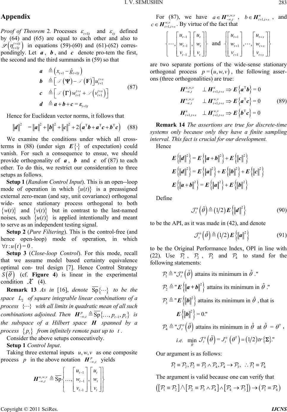 I. V. SEMUSHIN Copyright © 2011 SciRes. IJCNS 283 Appendix Proof of Theorem 2. Processes 1| tt and |tt defined by (64) and (65) are equal to each other and also to | 1| tst tt S in equations (59)-(60) and (61)-(62) corres- pondingly. Let a, b, and c denote pro-tem the first, the second and the third summands in (59) so that 11| 1 11 1| ˆ = ttt ts t tsts tt tt xg u wv FFF FS a b c dabcε (87) Hence for Euclidean vector norms, it follows that 2222 TTT =2 dabcabacbc (88) We examine the conditions under which all cross- terms in (88) (under sign E of expectation) could vanish. For such a consequence to ensue, we should provide orthogonality of a, b and c of (87) to each other. To do this, we restrict our consideration to three setups as follows. Setup 1 (Random Control Input). This is an open--loop mode of operation in which ()ut is a preassigned external zero-mean (and say, unit covariance) orthogonal wide- sence stationary process orthogonal to both ()wt and ()vt but in contrast to the last-named noises, such ()ut is applied intentionally and meant to serve as an independent testing signal. Setup 2 (Pure Filtering). This is the control-free (and hence open-loop) mode of operation, in which :=0tut. Setup 3 (Close-loop Control). For this mode, recall that we assume model based certainty equivalence optimal con- trol design [7]. Hence Control Strategy S (cf. Figure 4) is linear in the experimental condition X (4). Remark 13 As in [16], denote Sp to be the space 2 L of square integrable linear combinations of a process {} with all limits in quadratic mean of all such combinations adjoined. Then ,1 Sp ,, p ttt pp H is the subspace of a Hilbert space spanned by a process t p from infinitely remote past up to t. Consider the above setups consecutively. Setup 1 Control Input. Taking three extern al inputs ,,uwv as one composite process p in the above notation , p t H yields 1 ,, ,1 1 Sp ,, tt uwv ttt tt uu ww vv H For (87), we have ,, , uwv t a H, 1, u tts b H, and , 1, wv tts c H. By virtue of the fact that 1 1 1 ,, tt tt tt uu ww vv and 1 1 1 ,, tts tts tts uu ww vv are two separate portions of the wide-sense stationary orthogonal process =,,puwv , the following asser- ons (three orthogonalities) are true: ,, T ,1, ,, ,T ,1, ,T 1, 1, =0 =0 =0 uwvu ttts uwvwv ttts uwv tts tts HHEab HH Eac HHEbc (89) Remark 14 The assertions are true for discrete-time systems only because only they have a finite sampling interval. This fact is crucial for our development. Hence 222 2222 222 = = = EdEab Ec dEaEbEc EabEa Eb Define 2 aˆ12 t d (90) to be the API, as it was made in (42), and denote 2 oˆ12 t a (91) to be the Original Performance Index, OPI in line with (22). Use 1 , 2 , 3 and 4 to stand for the following statements: a 1 2 2 2 3 2 ˆˆ " attains its minimum i n ." ˆ " atta ins its minimum in ." ˆ " attains its m inimum in ,tha t is =0." t Ea+b Eb Eb o 4ˆˆˆ " attains its minimum in at = t † , i.e. oo ˆ= min tt †12 ."tr Our argument is as follows: 122344 314 ,,, The argument is valid because one can verify that 122344 314 ∧  I. V. SEMUSHIN Copyright © 2011 SciRes. IJCNS 284 is a tautology. Three premises (they are in brackets) are always TRUE. The first premise, 12 is TRUE because 2 cE is constant in ˆ . The second premise, 234 follows from the properties of norms, and the third premise, 43 is TRUE due to uniqueness of Kalman filter parameters when optimized in terms of criterion (22). Since the conclusion 14 is TRUE, this com- pletes the proof for Setup 1: criteria (90) and (91) are equimodal (have the same minimizing arguments). Setup 2 Pure Filtering. This mode eliminates b from ( 87) . For ter ms of (87), we have ,, wv t aH, =0b, and , 1, wv tts cH . By virtue of the fact that ,, ,1, wv wv ttts HH , we obtain T=0 Eac and 222 dEaEc. It means, together with definitions (40), (90) and (91) that ao 2 ˆˆ =const const=12 tt c E (92) and again, we are done. Setup 3 Close-loop Control. Consider Level 2 of uncertainty as acting in this setup. This is tantamount to stating that identification of is not needed. As in Setup 2, we observe that ,, wv t aH , =0b, and , 1, wv tts cH . The orthogonality ,, ,1, wv wv ttts HH (and as a result, T=0 Eac ) is true since 1 1 ,, tt tt ww vv and 1 1 ,, tts tts ww vv are two separate portions of the zero-mean orthogonal wide-sence stationaly process (,)wv . In order to get a deeper insight into the basic relation (92) and the conclusion “14 is TRUE”, let us look at them from some other point of view. Let a, b, and c denote pro-tem the first, the second and the third summands in (60) so that 1| 1| 1 |1 1| 1| ˆ [] = tt tt ts t tsts tt tt xg u FF P a bF cG dabcε (93) We are interested in b to vanish and in eliminating all cross-terms of (88) and its innovation analogue 2222 TTT =2 dabcabacbc (94) Innovation form (93) reinforces the fact that innovation version of the system (only if not in Setup 1) has the only “external” (better to say a hidden external) input. This is the innovation process |1tt , which is linear, or- thogonal and wide-sense stationary with the 1|2| 1 Sp ,, tt tt forming ,t H. The above outlined additional input {} t u appears in Setup 1. Starting from (93), we revisit the same setups: • Setup 1 Random Control Input. We observe that ,, u t aH , 1, u tts bH , 1,tts cH where 1 ,,12 1 Sp ,, tt u t tt tt uu vv H. By this, the following assertions are true: ,,1, ,T ,1, T 1, 1, =0 =0 =0 uu T ttts u ttts u ttstts HHEab HHEac HHEbc (95) Hence 222 2222 222 = = = EdEa+bEc EdEaEbEc Ea+bEa Eb Denote 2 oˆ12 tE a (96) to be another Original Performance Index, OPI' and add 2 and 4 to stand for the following statements: 2 2ˆ " attains its minimum in ." Eab o 4ˆˆˆ "attains its minimum i n at = ' t †, i.e. oo ˆ = min '' tt †=0." Consider them together with the above statements 1 2 3 2 ˆˆ "attains its minimum in ." ˆ " attains its minimu m in , that is 0." a t Eb Eb The following argument 1223443 14 ,,, is valid because 122 3443 14 is a tautology. All premises (placed in brackets) are always TRUE. The premise 12 is TRUE because  I. V. SEMUSHIN Copyright © 2011 SciRes. IJCNS 285 2 Ec is constant in ˆ . The premise 234 follows from the properties of norms. The third premise, 43 is TRUE due to uniqueness of Kalman filter parameters when optimized in terms of criterion (22). By the conclusion 14 being TRUE, the proof for Setup 1 is completed: criteria (90) and (96) have the same minimizing argument: † ˆ= . • Setup 2 Pure Filtering. In this case, ,t aH , =0b, 1,tts cH . By virtue of the fact that ,1,ttts HH , we obtain T=0 Ea c and 2Ed 222 dEaEc. It means, together with definitions (40), (90) and (96) that a 2 ˆˆ =const const=12 o tt Ec (97) Again, the conclusion 14 is TRUE for S e tup 2. • Setup 3 Closed-loop Control. In this case we are in the same situation: ,t aH , =0b, 1,tts cH . The conclusion 14 is TRUE for Setup 3, as well. Thus Theorem 2 is true.
|