Int. J. Communications, Network and System Sciences, 2011, 4, 232-240
doi:10.4236/ijcns.2011.44028 Published Online April 2011 (http://www.SciRP.org/journal/ijcns)
Empirical Modeling and Simulation of Temporal Based
Adaptive Mobility Model for MANET
Gurusamy Prema1,3, Chandrabose Aravindan2, Kirthivasan Kannan1, Rathinam Maheswaran3
1SASTRA University, Thanjavur, India
2SSN College of Engineering, Chennai, India
3Mepco Schlenk Engineering College, Sivak as i, India
Received December 14, 2010; revised February 20, 2011; accepted February 28, 2011
Abstract
Mobile Ad Hoc network (MANET) is a collection of wireless mobile nodes forming a temporary network
without the aid of any established infrastructure. To conduct meaningful performance analysis of MANETs,
it is essential that the simulation of mobility model should reflect the realistic mobility pattern of mobile
nodes i.e. placement of mobile nodes at different intervals of time. The formation of spontaneous network
depends heavily on the movement of different nodes in a particular practical scenario. This research focuses
on the modeling and simulation of a temporal Adaptive Mobility Model which can be adapted to any dy-
namic practical scenario. The mobility in the realistic environment is simulated based on a Probability Tran-
sition Matrix named as Personal Behavior Model (PBM) and validated for a practical Health Care Environ-
ment. The formation of MANET is assumed to be based on the movement of the patient i.e. mobile nodes in
the health care environment. Patients waiting in front of each service point for different time intervals are
taken as results and compared with the actual data.
Keywords: MANET, Mobility Model, Probability Transition Matrix, System Dynamics
1. Introduction
A Mobile Ad Hoc Network (MANET) is a spontaneous,
self-organizing network of mobile computing devices,
having no fixed infrastructure or administrative support,
where each mobile node also acts as a router of network
packets. The primary function of the MANET is to fa-
cilitate communication between its cons tituen t nod es. So,
each node on the network may be either sender or re-
ceiver of packets, and all nodes works as router as dis-
cussed in [1]. MANET’s performance is validated by
simulation with the help of mobility models that describe
and dictate the mobility pattern of the mobile nodes that
take part in forming MANET. Mobility mode l mimic the
movement of mobile nodes in MANET simulation and is
a representation of a certain real or abstract world that
contains moving entities. The mobility model describes
the movement pattern of mobile user and how their loca-
tion, change over time. The movement pattern of mobile
nodes plays an important role in the performance analy-
sis of wireless networks [2,3]. The mobility of the nodes
affects the number of average connected paths, which in
turn affect the performance of the routing algorithm [4].
In [5], S.Ray discussed some of the mobility models are
realistic and they reflect as close as possible those real
world scenarios.
Due to the dynamic nature of users in a MANET, a
key challenge in the evaluation of mobility pattern is to
conduct the performance analysis, with realistic mobility
models that accurately reflect the mobile users’ move-
ment [6]. In their work, S.Gowrishankar et al. discussed
about MANET environment, where mobile nodes are
free to join or leave the network at any point of time,
resulting in a highly dynamic netwo rk environment com-
pare to wired network [7]. The advantage and importance
of simulation of mobility model for MANET is discussed
in [8]. Several mobility models have been developed for
MANET simulations and mostly they are unrealistic mo-
bility models. In the unrealistic mobility model, the node
can move towards a randomly chosen destination with a
randomly chosen speed and direction [9]. They are not
suitable for real environment. In realistic mobility mod-
els, the node can move towards proper destination in-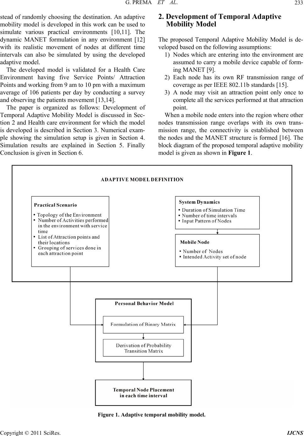

G. PREMA ET AL.233
stead of randomly choosing the destination. An adaptive
mobility model is developed in this work can be used to
simulate various practical environments [10,11]. The
dynamic MANET formulation in any environment [12]
with its realistic movement of nodes at different time
intervals can also be simulated by using the developed
adaptive model.
The developed model is validated for a Health Care
Environment having five Service Points/ Attraction
Points and working from 9 am to 10 pm with a maximum
average of 106 patients per day by conducting a survey
and observing the patients movement [13,14].
The paper is organized as follows: Development of
Temporal Adaptive Mobility Model is discussed in Sec-
tion 2 and Health care environment for which the model
is developed is described in Section 3. Numerical exam-
ple showing the simulation setup is given in Section 4.
Simulation results are explained in Section 5. Finally
Conclusion is given in Section 6.
2. Development of Temporal Adaptive
Mobility Model
The proposed Temporal Adaptive Mobility Model is de-
veloped based on the following assumptions:
1) Nodes which are entering into the environment are
assumed to carry a mobile device capable of form-
ing MANET [9].
2) Each node has its own RF transmission range of
coverage as per IEEE 802.11b standards [15].
3) A node may visit an attraction point only once to
complete all the servic es perf ormed at that a ttract io n
point.
When a mobile node enters into the region where other
nodes transmission range overlaps with its own trans-
mission range, the connectivity is established between
the nodes and the MANET structure is formed [16]. The
block diagram of the proposed temporal adaptive mobility
model is given as shown in Figure 1.
Figure 1. Adaptive temporal mobility model.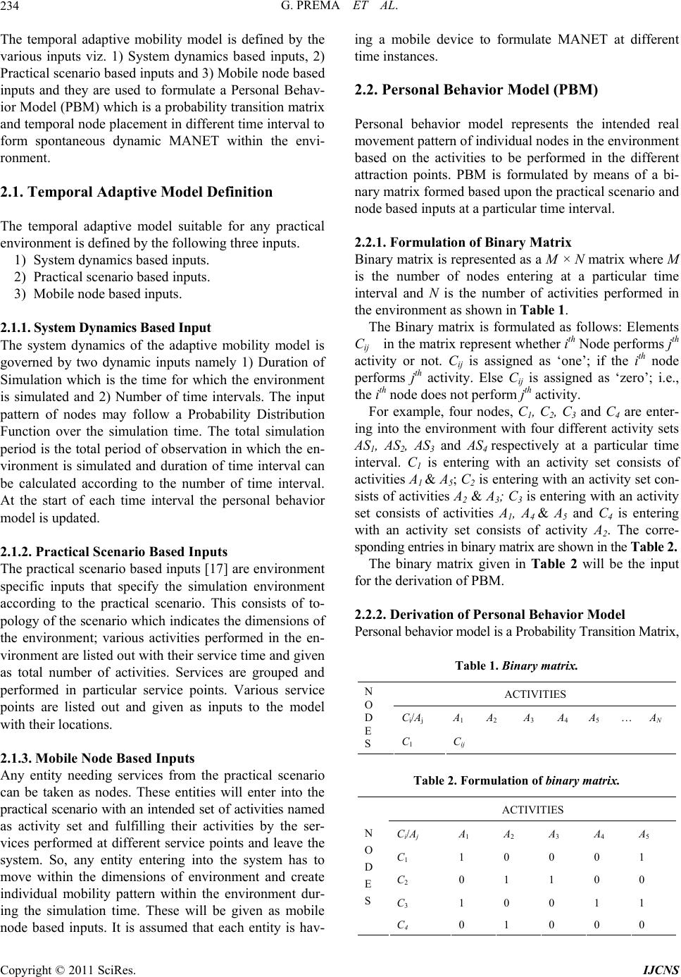

G. PREMA ET AL. 234
The temporal adaptive mobility model is defined by the
various inputs viz. 1) System dynamics based inputs, 2)
Practical scenario based inputs and 3) Mobile node based
inputs and they are used to formulate a Personal Behav-
ior Model (PBM) which is a probability transition matrix
and temporal node placement in different time interval to
form spontaneous dynamic MANET within the envi-
ronment.
2.1. Temporal Adaptive Model Definition
The temporal adaptive model suitable for any practical
environment is defined by the following three inputs.
1) System dynamics based inputs.
2) Practical scenario based inputs.
3) Mobile no de b a sed i np uts .
2.1.1. System Dynamics Based Input
The system dynamics of the adaptive mobility model is
governed by two dynamic inputs namely 1) Duration of
Simulation which is the time for which the environment
is simulated and 2) Number of time intervals. The input
pattern of nodes may follow a Probability Distribution
Function over the simulation time. The total simulation
period is the total period of observation in which the en-
vironment is simulated and duration of time interval can
be calculated according to the number of time interval.
At the start of each time interval the personal behavior
model is updated.
2.1.2. Practical Scenario Based Inputs
The practical scenario based inputs [17] are environment
specific inputs that specify the simulation environment
according to the practical scenario. This consists of to-
pology of the scenario which indicates the dimensions of
the environment; various activities performed in the en-
vironment are listed out with their service time and given
as total number of activities. Services are grouped and
performed in particular service points. Various service
points are listed out and given as inputs to the model
with their locations.
2.1.3. Mobile Node Based Inputs
Any entity needing services from the practical scenario
can be taken as nodes. These entities will enter into the
practical scena rio with an intended set o f activities named
as activity set and fulfilling their activities by the ser-
vices performed at different service points and leave the
system. So, any entity entering into the system has to
move within the dimensions of environment and create
individual mobility pattern within the environment dur-
ing the simulation time. These will be given as mobile
node based inputs. It is assumed that each entity is hav-
ing a mobile device to formulate MANET at different
time instances.
2.2. Personal Behavior Model (PBM)
Personal behavior model represents the intended real
movement pattern of individual nodes in the environment
based on the activities to be performed in the different
attraction points. PBM is formulated by means of a bi-
nary matrix formed based upon the practical scenario and
node based inputs at a particular time interval.
2.2.1. Formulation of Binary Matrix
Binary matrix is represented as a M × N matrix where M
is the number of nodes entering at a particular time
interval and N is the number of activities performed in
the environment as shown in Table 1.
The Binary matrix is formulated as follows: Elements
Cij in the matrix represent whether ith Node performs jth
activity or not. Cij is assigned as ‘one’; if the i
th node
performs jth activity. Else Cij is assigned as ‘zero’; i.e.,
the ith node does not perform jth activity.
For example, four nodes, C1, C2, C3 and C4 are enter-
ing into the environment with four different activity sets
AS1, AS2, AS3 and AS4 respectively at a particular time
interval. C1 is entering with an activity set consists of
activities A1 & A5; C2 is en tering with an activity set con-
sists of activities A2 & A3; C3 is entering with an activity
set consists of activities A1, A4 & A5 and C4 is entering
with an activity set consists of activity A2. The corre-
sponding entries in binary matrix are shown in the Table 2.
The binary matrix given in Table 2 will be the input
for the derivation of PBM.
2.2.2. Derivation of Personal Behavior Model
Personal behavior model is a Probability Transition Matrix,
Table 1. Binary matrix.
ACTIVITIES
Ci/Aj A1 A2 A3 A4 A5 …AN
N
O
D
E
S C1 Cij
Table 2. Formulation of binary matrix.
ACTIVITIES
Ci/Aj A1 A2 A3 A4 A5
C1 1 0 0 0 1
C2 0 1 1 0 0
C3 1 0 0 1 1
N
O
D
E
S
C4 0 1 0 0 0

G. PREMA ET AL.235
which indicates the probable movement of the nodes to
fulfill the intended activities towards various service
points in the environment. The matrix is having dynamic
rows based upon the nodes available in the system other
than waiting in front of the attraction points and number
of attraction points as columns and updated at the start-
ing of each time interval. This behavior model is used to
denote the Probab ility of the nodes moving towards each
attraction point. The Personal behavior model is derived
as follows: Let Ti be the total number of activities in the
intended activity set of the ith node and Tik be the number
of activities serviced in kth attraction point for ith node.
Probability P(Ci, APk) represents the probability of ith
node in the system intended to move to the kth attraction
point and given by the Equation (1).

,ik
ik i
T
PC APT  (1)
For a particular time interval, having the binary matrix
as shown in Table 2, the PBM is derived as shown in
Table 3.
Consider a practical environment, where there are
three attraction points lo cated and activities A1 and A2 are
performed in AP1, activities A3 and A5 are performed in
AP2 and activity A4 is performed in AP3. For the binary
matrix shown in Table 3, the entries in the PBM are as
shown in Table 4.
After completion of all the activities, a node will move
to next attraction point if it is having activity to do and
after completing all the intended activities a node will
leave the system.
Table 3. Formulation of personal behavior model.
Attraction Points
Ci/APk AP1 AP3 … APP
C1
…
N
O
D
E
S
CN
P(Ci,APk)
Table 4. Personal behavior model.
Attraction Points
Ci/APk AP1 AP2 AP3
C1 0.5 0.5 0
C2 0 1 0
C3 0.33
0.33 0.33
N
O
D
E
S
C4 1 0 0
2.3. Temporal Node Placement
For a given simulation time, different nodes are entering
into the system and move according to their intended
activity set. For any discrete time interval of the simula-
tion, the nodes will be distributed over the entire dimen-
sions of the environment. This distribution is purely
based upon purpose of entering the system and leaving
the system after the services are completed. So, the con-
nectivity of the nodes will be spontaneous and it will
form a self organizing network i.e. MANET. So, the
node placement during the entire simulation time is taken
as the mobility pattern of the system to formulate the
MANET structure.
3. Health Care Environment
The Temporal adaptive mobility model develop ed is tes-
ted for a practical health care environment, where 31
different activities are performed at 5 different service
points namely, Doctor’s Room, Injection/Dressing Room,
Pharmacy, Laboratory and Physiotherapy centre and is
working from 9 a.m to 10 p.m. After making a pilot sur-
vey for a period of one month, it is observed that a
maximum average of 106 patients is entering into the
system to avail different services.
Health care environment is defined by having the sys-
tem dynamic based inputs, the total simulation period
780 minutes is divided into 26 numbers of equal intervals,
each of 30 minutes duration. First interval is from 9.00
am to 9.30 am, second interval is from 9.30 am to 10.00
am, etc. up to 26th interval is from 9.30 pm to 10 pm. It is
assumed that Personal Behavior Matrix is updated at the
start of each time interval. For the first time interval it is
updated at 9.00 am, second time at 9.30 am etc. The Ar-
rival pattern of the nodes into the system may follow a
probability distribu tion and observed during th e different
time intervals is plotted as shown in Figure 2.
Figure 2. Number of nodes entered into the system in each
time interval.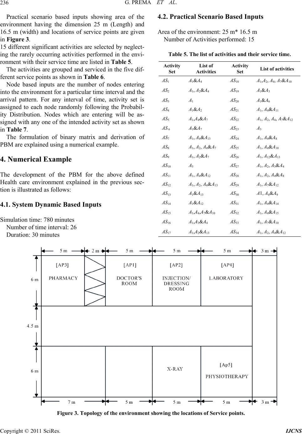

G. PREMA ET AL. 236
4.2. Practical Scenario Based Inputs Practical scenario based inputs showing area of the
environment having the dimension 25 m (Length) and
16.5 m (width) and locations of service points are given
in Figure 3. Area of the environment: 25 m* 16.5 m Number of Activities performed: 15
15 different significant activities are selected by neglect-
ing the rarely occurring activities performed in the envi-
ronment with their service time are listed in Table 5. Table 5. The list of activities and their service time.
Activity
Set List of Activities Activity Set List of activities
AS1 A1&A4 AS18 A1,A2, A4, A7&A10
AS2 A1, A2&A4 AS19 A1&A3
AS3 A1 AS20 A1&A6
AS4 A1&A2 AS21 A1, A4&A11
AS5 A1,A4&A7 AS22 A1, A2, A4, A7&A12
AS 6 A1&A7 AS23 A3
AS7 A1, A4&A13 AS24 A1, A4&A8
AS8 A1, A2, A4&A7 AS25 A1, A4&A10
AS9 A1, A2&A7 AS26 A1, A12&A13
AS10 A5 AS27 A1, A2, A3&A4
AS11 A1, A4&A12 AS28 A1, A2, A4&A8
AS12 A1, A2, A4&A13 AS29 A1, A7&A12
AS13 A1&A13 AS30 A1, A4&A9
AS14 A1&A12 AS31 A1, A4&A14
AS15 A1,A4,A7&A10 AS32 A1, A4&A15
AS16 A1,A3&A4 AS33 A1, A7&A10
AS17 A1,A2&A13 AS34 A1, A2, A4&A12
The activities are grouped and serviced in the five dif-
ferent service points as shown in Table 6.
Node based inputs are the number of nodes entering
into the environment for a particular time interval and the
arrival pattern. For any interval of time, activity set is
assigned to each node randomly following the Probabil-
ity Distribution. Nodes which are entering will be as-
signed with any one of the intended activity set as shown
in Table 7.
The formulation of binary matrix and derivation of
PBM are explained using a numerical example.
4. Numerical Example
The development of the PBM for the above defined
Health care environment explained in the previous sec-
tion is illustrated as follows:
4.1. System Dynamic Based Inputs
Simulation time: 780 minutes
Number of time interval: 26
Duration: 30 minutes
Figure 3. Topology of the environment showing the locations of Service points.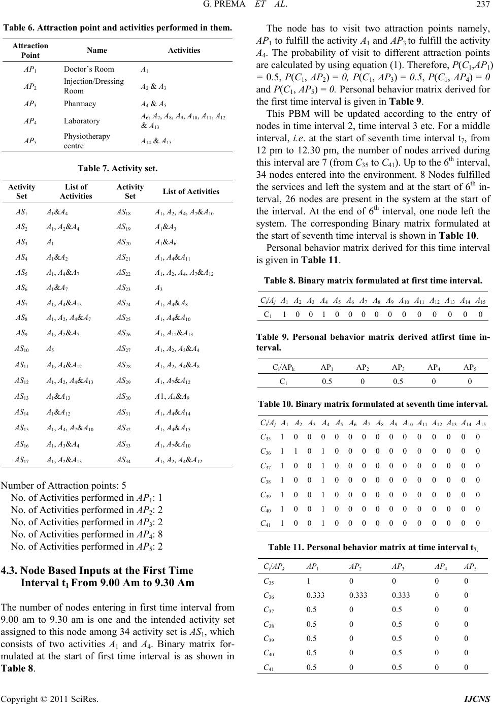

G. PREMA ET AL. 237
Table 6. Attraction point and activities performed in them.
Attraction
Point Name Activities
AP1 Doctor’s Room A1
AP2 Injection/Dressing
Room A2 & A3
AP3 Pharmacy A4 & A5
AP4 Laboratory A6, A7, A8, A9, A10, A11, A12
& A13
AP5 Physiotherapy
centre A14 & A15
Table 7. Activity set.
Activity
Set List of Activities Activity Set List of Activities
AS1 A1&A4 AS18 A1, A2, A4, A7&A10
AS2 A1, A2&A4 AS19 A1&A3
AS3 A1 AS20 A1&A6
AS4 A1&A2 AS21 A1, A4&A11
AS5 A1, A4&A7 AS22 A1, A2, A4, A7&A12
AS6 A1&A7 AS23 A3
AS7 A1, A4&A13 AS24 A1, A4&A8
AS8 A1, A2, A4&A7 AS25 A1, A4&A10
AS9 A1, A2&A7 AS26 A1, A12&A13
AS10 A5 AS27 A1, A2, A3&A4
AS11 A1, A4&A12 AS28 A1, A2, A4&A8
AS12 A1, A2, A4&A13 AS29 A1, A7&A12
AS13 A1&A13 AS30 A1, A4&A9
AS14 A1&A12 AS31 A1, A4&A14
AS15 A1, A4, A7&A10 AS32 A1, A4&A15
AS16 A1, A3&A4 AS33 A1, A7&A10
AS17 A1, A2&A13 AS34 A1, A2, A4&A12
Number of Attraction points: 5
No. of Activities performed in AP1: 1
No. of Activities performed in AP2: 2
No. of Activities performed in AP3: 2
No. of Activities performed in AP4: 8
No. of Activities performed in AP5: 2
4.3. Node Based Inputs at the First Time
Interval t1 From 9.00 Am to 9.30 Am
The number of nodes entering in first time interval from
9.00 am to 9.30 am is one and the intended activity set
assigned to this node among 34 activity set is AS1, which
consists of two activities A1 and A4. Binary matrix for-
mulated at the start of first time interval is as shown in
Table 8.
The node has to visit two attraction points namely,
AP1 to fulfill the activity A1 and AP3 to fulfill the activity
A4. The probability of visit to different attraction points
are calculated by using equation (1). Therefore, P(C1,AP1)
= 0.5, P(C1, AP2) = 0, P(C1, AP3) = 0.5, P(C1, AP4) = 0
and P(C1, AP5) = 0. Personal behavior matrix derived for
the first time interval is given in Table 9.
This PBM will be updated according to the entry of
nodes in time interval 2, time interval 3 etc. For a middle
interval, i.e. at the start of seventh time interval t7, from
12 pm to 12.30 pm, the number of nodes arrived during
this interval are 7 (from C35 to C41). Up to the 6th interval,
34 nodes entered into the environment. 8 Nodes fulfilled
the services and left the system and at the start of 6th in-
terval, 26 nodes are present in the system at the start of
the interval. At the end of 6th interval, one node left the
system. The corresponding Binary matrix formulated at
the start of seventh time interval is shown in Table 10.
Personal behavior matrix derived for this time interval
is given in Table 11.
Table 8. Binary matrix formulated at first time interval.
Ci/AjA1A2A3A4A5A6A7A8 A9 A10 A11 A12 A13 A14 A15
C110010000 0 0 0 0 000
Table 9. Personal behavior matrix derived atfirst time in-
terval.
Ci/APk AP1 AP2 AP3 AP4 AP5
C1 0.5 0 0.5 0 0
Table 10. Binary matrix formulated at seventh time interval.
Ci/AjA1A2A3A4A5A6A7 A8 A9 A10 A11 A12 A13 A14 A15
C35 10000000 0 0 0 0 000
C36 11010000 0 0 0 0 000
C37 10010000 0 0 0 0 000
C38 10010000 0 0 0 0 000
C39 10010000 0 0 0 0 000
C40 10010000 0 0 0 0 000
C41 10010000 0 0 0 0 000
Table 11. Personal behavior matrix at time interval t7.
Ci/APk AP1 AP2 AP3 AP4 AP5
C35 1 0 0 0 0
C36 0.333 0.333 0.333 0 0
C37 0.5 0 0.5 0 0
C38 0.5 0 0.5 0 0
C39 0.5 0 0.5 0 0
C40 0.5 0 0.5 0 0
C41 0.5 0 0.5 0 0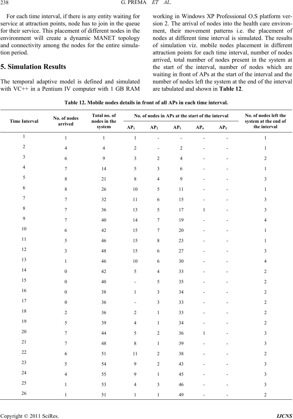

G. PREMA ET AL. 238
For each time interval, if there is any entity waiting for
service at attraction points, node has to join in the queue
for their service. This placement of different nodes in the
environment will create a dynamic MANET topology
and connectivity among the nodes for the entire simula-
tion peri od.
5. Simulation Results
The temporal adaptive model is defined and simulated
with VC++ in a Pentium IV computer with 1 GB RAM
working in Windows XP Professional O.S platform ver-
sion 2. The arrival of nodes into the health care environ-
ment, their movement patterns i.e. the placement of
nodes at different time interval is simulated. The results
of simulation viz. mobile nodes placement in different
attraction points for each time interval, number of nodes
arrived, total number of nodes present in the system at
the start of the interval, number of nodes which are
waiting in front of APs at the start of the interval an d the
number of nodes left the system at the end of th e interval
are tabulated and show n in Table 12.
Table 12. Mobile nodes details in front of all APs in each time interval.
No. of nodes in APs at the start of the interval
Time Interval No. of nodes
arrived
Total no. of
nodes in the
system AP1 AP2 AP3 AP4 AP5
No. of nodes left the
system at the end of
the interval
1 1 1 1 - - - - 1
2 4 4 2 - 2 - - 1
3 6 9 3 2 4 - - 2
4 7 14 5 3 6 - - 1
5 8 21 8 4 9 - - 3
6 8 26 10 5 11 - - 1
7 7 32 11 6 15 - - 3
8 7 36 13 5 17 1 - 3
9 7 40 14 7 19 - - 4
10 6 42 15 7 20 - - 1
11 5 46 15 8 23 - - 1
12 3 48 15 6 27 - - 3
13 1 46 10 6 30 - - 4
14 0 42 5 4 33 - - 2
15 0 40 - 5 35 - - 2
16 0 38 1 3 34 - - 2
17 0 36 - 3 33 - - 2
18 2 36 2 1 33 - - 2
19 5 39 4 1 34 - - 2
20 7 44 5 2 36 1 - 3
21 7 48 8 1 39 - - 3
22 6 51 11 2 38 - - 2
23 5 54 9 2 43 - - 3
24 4 55 9 1 45 - - 3
25 1 53 4 3 46 - - 3
26 1 51 1 1 49 - - 2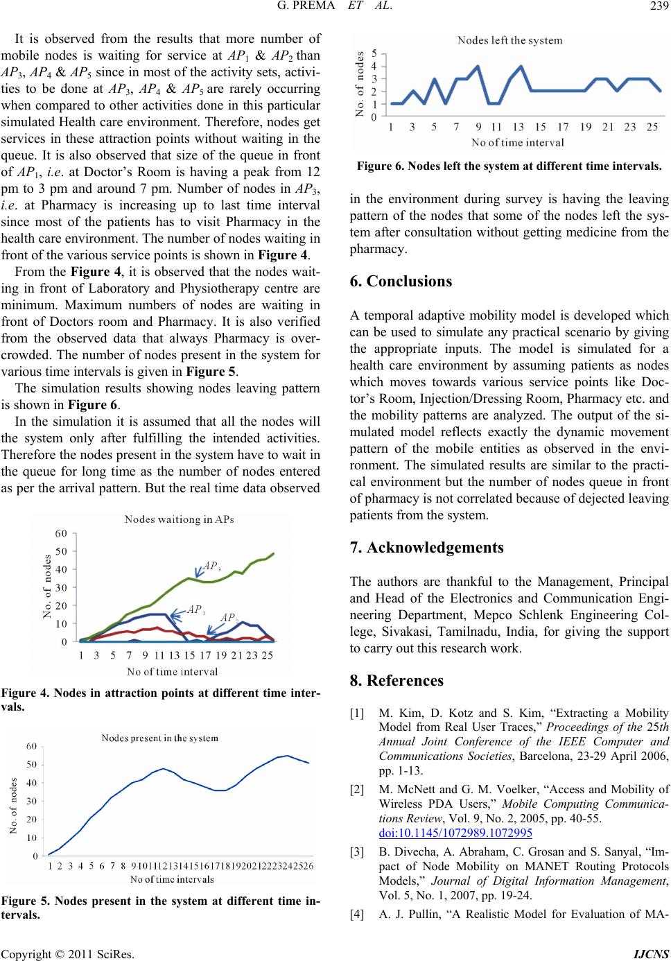

G. PREMA ET AL. 239
It is observed from the results that more number of
mobile nodes is waiting for service at AP1 & AP2 than
AP3, AP4 & AP5 since in most of the activ ity sets, activi-
ties to be done at AP3, AP4 & AP5 are rarely occurring
when compared to other activities done in this particular
simulated Health care environment. Therefore, nodes get
services in these attraction points without waiting in the
queue. It is also observed that size of the queue in front
of AP1, i.e. at Doctor’s Room is having a peak from 12
pm to 3 pm and around 7 pm. Number of nodes in AP3,
i.e. at Pharmacy is increasing up to last time interval
since most of the patients has to visit Pharmacy in the
health care environment. The number of nodes waitin g in
front of the various service points is shown in Figure 4.
From the Figure 4, it is observed that the nodes wait-
ing in front of Laboratory and Physiotherapy centre are
minimum. Maximum numbers of nodes are waiting in
front of Doctors room and Pharmacy. It is also verified
from the observed data that always Pharmacy is over-
crowded. The number of nodes present in the system for
various time intervals is given in Figure 5.
The simulation results showing nodes leaving pattern
is shown in Figure 6.
In the simulation it is assumed that all the nodes will
the system only after fulfilling the intended activities.
Therefore the nodes pr esent in the system hav e to wait in
the queue for long time as the number of nodes entered
as per the arrival pattern. But the real time data observed
Figure 4. Nodes in attraction points at different time inter-
vals.
Figure 5. Nodes present in the system at different time in-
tervals.
Figure 6. Nodes left the system at different time intervals.
in the environment during survey is having the leaving
pattern of the nodes that some of the nodes left the sys-
tem after consultation without getting medicine from the
pharmacy.
6. Conclusions
A temporal adaptive mobility model is developed which
can be used to simulate any practical scenario by giving
the appropriate inputs. The model is simulated for a
health care environment by assuming patients as nodes
which moves towards various service points like Doc-
tor’s Room, Injection/Dressing Room, Pharmacy etc. and
the mobility patterns are analyzed. The output of the si-
mulated model reflects exactly the dynamic movement
pattern of the mobile entities as observed in the envi-
ronment. The simulated results are similar to the practi-
cal environment but the number of nodes queue in front
of pharmacy is not correlated because of dejected leaving
patients from the system.
7. Acknowledgements
The authors are thankful to the Management, Principal
and Head of the Electronics and Communication Engi-
neering Department, Mepco Schlenk Engineering Col-
lege, Sivakasi, Tamilnadu, India, for giving the support
to carry out this research work.
8. References
[1] M. Kim, D. Kotz and S. Kim, “Extracting a Mobility
Model from Real User Traces,” Proceedings of the 25th
Annual Joint Conference of the IEEE Computer and
Communications Societies, Barcelona, 23-29 April 2006,
pp. 1-13.
[2] M. McNett and G. M. Voelker, “Access and Mobility of
Wireless PDA Users,” Mobile Computing Communica-
tions Review, Vol. 9, No. 2, 2005, pp. 40-55.
doi:10.1145/1072989.1072995
[3] B. Divecha, A. Abraham, C. Grosan and S. Sanyal, “Im-
pact of Node Mobility on MANET Routing Protocols
Models,” Journal of Digital Information Management,
Vol. 5, No. 1, 2007, pp. 19-24.
[4] A. J. Pullin, “A Realistic Model for Evaluation of MA-

G. PREMA ET AL. 240
NET,” Proceedings of Innovation North Research &
Practice Conference, Leeds, 9-11 July 2007, pp. 1-15.
[5] S. Ray, “Realistic Mobility for MANET Simulation,”
Master’s Thesis, The University of British Columbia,
Vancouver, 2003.
[6] A. Jardosh, E. M. Belding-Royer, K. C. Almeroth and S.
Suri, “Real World Environment Models for Mobile Ad-
Hoc Networks Evaluation,” IEEE Journal on Selected
Areas in Communications, Special Issue on Wireless Ad
Hoc Networks, Vol. 23, No. 3, 2005, pp. 622-632.
[7] S. Gowrishankar, T. G. Basavaraju and S. Sarkar, “Effect
of Random Mobility Models Pattern in Mobile Ad Hoc
Networks,” International Journal of Computer Science
and Network Security, Vol. 7, No. 6, 2007, pp. 160-164.
[8] P. Venkateswaran, R. Ghosh, A. Das, S. K. Sanyal and R.
Nandi, “An Obstacle Based Realistic Ad-Hoc Mobility
Model for Social Networks,” Journal of Networks, Vol. 1,
No. 2, 2006, pp. 37-44.
[9] T. Camp, J. Boleng and V. Davies, “A Survey of Mobil-
ity Models for Ad Hoc Network Research,” Wireless
Communication and Mobile Computing: Special Issue on
Mobile Ad Hoc Networking: Research, Trends and Appli-
cations, Vol. 2, No. 5 , 2002, pp. 483-502.
[10] A. J. Pullin and C. Pattinson, “A Realistic Battlefield
Model for the Evaluation of MANET,” Proceedings of
5th Annual Conference on Wireless on Demand Network
Systems and Services, Garmisch Partenkirchen, 23-25
January 2008, Vol. 23, pp. 81-84.
doi:10.1109/WONS.2008.4459359
[11] T. M. L. Flower, G. Prema, C. Aravindan, K. Kannan and
R. Maheswaran, “A Realistic Mobility Pattern for Adap-
tive MANET Simulation Environment,” Proceedings of
National Conference on Networks, Image & Security,
Kumarakoil, 14-15 March 2008, pp. 70-75.
[12] G. Lu, G. Manson and D. Belis, “Mobility Modeling in
Mobile Ad Hoc Networks with Environment-Aware,”
Journal of Networks, Vol. 1, No. 1, 2006, pp. 54-63.
[13] D. Bhattacharjee, A. C. R. Shah, M. Shah and A. Helmy,
“Empirical Modeling of Campus-Wide Pedestrian Mobil-
ity: Observations on the USC Campus,” Proceedings of
IEEE Vehicular Technology Conference, Los Angeles, 26-
29 September 2004 Vol. 4, pp. 2887-2891.
[14] J. Kim and S. Bohacek, “A Survey-Based Mobility Mod-
el of People for Simulation of Urban Mesh Networks,”
Proceedings of Mesh Nets, Budapest, July 2005, pp. 1-11.
[15] D. Huang, “Unlinkability Measure for IEEE 802.1 1 Based
MANETs,” IEEE Transactions on Wireless Communica-
tions, Vol. 7, No. 2, 2008, pp. 1025-1034.
doi:10.1109/TWC.2008.060777
[16] M. A. Rajan, M. G. Chandra, L. C. Reddy and P. S. Hi-
remath, “Topological and Energy Analysis of K-Con-
nected MANETs: A Semi-Analytical Approach,” Inter-
national Journal of Computer Science and Network Se-
curity, Vol. 8, No. 2, 2008, pp. 199-207.
[17] P. Johansson, T. Larsson, N. Hedman, B. Mielczarek and
M. Degermark, “Scenario Based Performance Analysis of
Routing Protocols for Mobile Ad Hoc Networks,” Pro-
ceedings of the 5th ACM Annual International Confer-
ence on Mobile Computing and Networking, Seattle, 15-
19 August 1999, pp. 195-206.