 Journal of Applied Mathematics and Physics, 2014, 2, 397-404 Published Online May 2014 in SciRes. http://www.scirp.org/journal/jamp http://dx.doi.org/10.4236/jamp.2014.26047 How to cite this paper: Zhuang, Y. (2014) Novel Finite Difference Discretization of Interface Boundary Conditions for Stab- lized Explicit-Implicit Domain Decomposition Methods. Journal of Applied Mathematics and Physics, 2, 397-404. http://dx.doi.org/10.4236/jamp.2014.26047 Novel Finite Difference Discretization of Interface Boundary Conditions for Stablized Explicit-Implicit Domain Decomposition Methods Yu Zhuang Computer Science Department, Texas Tech University, Lubbock, Texas, USA Email: yu.zhuang@ttu.edu Received March 2014 Abstract Stabilized explicit-implicit domain decomposition is a group of methods for solving time-depen- dent partial difference equations of the parabolic type on parallel computers. They are efficient, stable, and highly parallel, but suffer from a restriction that the interface boundaries must not in- tersect inside the domain. Various techniques have been proposed to handle this restriction. In this paper, we present finite difference schemes for discretizing the equation spatially, which is of high simplicity, easy to implement, attains second-order spatial accuracy, and allows interface boundaries to intersect inside the domain. Keywords Domain Decomposition, Parallel Computing, Unsteady Convection-Diffusion Equation, Finite Difference 1. Introduction Convection-diffusion processes appear in many science and engineering studies, e.g. heat transfer-based engi- neering [1] [2] [3], pollution and waste treatment modeling [4] [5] [6], propagation of neuronal membrane po- tential [7] [8] [9] [10], the signaling mechanism of nitric oxide in and cardiovascular [11] and nervous [12] sys- tems. The governing equations of convection-diffusion processes have the general form ()( ) ( ) ( ) ( ) ( ) ,u ,Ωutxaxc xusxux t ∂=∇⋅∇ +∇⋅+∈ ∂ (1) with boundary condition (2) where is the spatial domain, is the boundary of the spatial domain, is the diffusion coefficient, 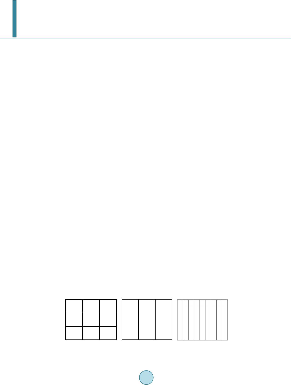 Y. Zhuang is the advection velocity, and is the source/sink term. Explicit implicit domain decomposition (EIDD) methods [13] [14] [15]-[17] [18] [19] [20] [21]-[27] [28] [ 29] [30]-[35] [36] [37] [38] are a class of glo- bally non-iterative, non-overlapping domain decomposition methods for solving Equation (1) and (2) on parallel computers, which are algorithmically simple, computationally and communicationally efficient. One group of EIDD methods achieves good stability with implicit correction of the explicitly predicted interface boundary conditions [15] [27] [28] [29] [30]-[35]. In parallel implementation of corrected EIDD methods, the correction step is communicationally expensive to be parallelized when the interior boundaries cross into each other inside the domain, e.g. as in Figure 1(a). While for some problems [10], it causes no trouble to partition a domain with no intersecting interior boundaries, in many cases corrected EIDD methods suffer from low accuracy when partitioned into a large number of nar- row strip subdomains when a large number of processors is used [34]. To address the problem of no crossover for interior boundaries, Shi and Liao [29] introduced in 2006 zigzag interior (ZI) boundaries so that in the impli- cit correction, spatial discretization does not result in coupling of all grip points on the interior boundaries into one single equation. In 2009, Liao, Shi, and Sun [27] developed composite interior boundaries by replacing the ZI boundaries in [29] with straight-line interior boundaries at locations neighboring intersection points of inte- rior boundaries, leading to improved programming simplicity for the treatment of interior boundaries than the ZI boundaries. Zhu, Yuan, and Du [30] [31] used a different technique to handle the crossover of interior bounda- ries. Jun and Mai [20] [39] used special treatment for the implicit discretization at points neighboring intersec- tion points while maintaining unconditional stability. The interface boundary treatment introduced by Jun and Mai for their modified implicit prediction method [20] [39] can also be used to solve the intersecting interior boundary problem for corrected EIDD methods. Zhuang and Sun [35] and Wang, Wu, and Zhuang [37] tackled disadvantages of no-crossover interface boundaries by using a data partition different from the domain partition, where the domain is partitioned with no crossover interface boundaries as in Figure 1(b) but the data of each subdoman is further partitioned into multiple data subsets like in Figure 1(a) for distribution to different pro- cessor s. To allow crossover of interface boundaries, in this paper we propose new finite difference schemes for inter- face boundary conditions at intersecting points of crossover interface boundaries. The technical motivation of this finite difference approximation is given in Section 2, which describes a Stabilized Explicit-Implicit Domain Decomposition Methods and the problems of the interface boundary condition treatment when standard finite different approximation is used. Section 3 describes the new finite different schemes for interface boundary conditions. In Section 4 we present numerical tests, and Section 5 gives the concluding remarks. 2. The Stabilized EIDD Method and Need for Interface Boundary Condition Treatment Stabilized EIDD (SEIDD) methods [34] [35] and the more general corrected EIDD (CEIDD) methods [15] [27] [28] [29] [30] -[35] are operator splitting time discretization methods for time dependent partial differential equ- ations, where operator splitting is domain decomposition-based. A common feature of the SEIDD and CEIDD methods that call for a communication-effic iency-targeting treatment of the interface boundary conditions is the stabilization or correction of the interface boundary conditions by an implicit time discretization scheme. To see how this technical issue arises, for reading convenience, we give the description of a SEIDD method below. To that end, we first list some notations. To numerically solve problem (1 - 2), we choose a discrete spatial grid Ωℎ with mesh size h, and discretize Equations (1) and (2) spatially into (a) (b) (c) Figure 1. Different ways of domain partitions.  Y. Zhuang ( )( ) ( ) 0 , 0, dut Aut dt uu = = (3) where is the discrete approximation of the spatial operator on the right hand side of Equation (1). Our de- scription will be based on this spatially discrete form of the equation. For a domain partitioned as in Figure 1(b) or Figure 1(c), let B be the set of grid points on interface boundaries. With denoting the numerical solution of the -th time step, the SEIDD method for computing the solution at the (k + 1)-th time step from the current k-th time step is given below. A SEIDD Method 1) Compute the interface boundary condition using the explicit forward Euler scheme on inter face boundaries points , where is the identity matrix. 2) Using the interface boundary conditions computed at step 1 together with exterior boundary conditions, compute the solution on the subdomains using the implicit backward Euler scheme . 3) Throw away the interface boundary condition computed at step 1. Using solution data on nearby sub- domain as boundary conditions, re-compute interface boundary condition on interface boundary with the backward Euler . A SEIDD method or a CEIDD method uses an implicit scheme, e.g. the backward Euler, to implicitly re- compute solution on the interface boundary . When the domain is partitioned with no intersection of interface boundaries, like in Figure 1(b) or Figure 1(c), the implicit re-computation of interface boundary con- dition on different interface boundaries can be executed by processors independently and hence in parallel when different interface boundaries are assigned to different processors. But when a domain is partitioned as in Figure 1(a), conventional finite difference approximation of Equation (1) on the interface boundaries would generate a discrete equation coupling all grid points on the interface boundaries, and since these interface boundary grid points are distributed on different processors, to solve a discrete equation involving all grid points of the inter- face boundaries would require expensive all-to-all communication. Domain partition with no crossover interface boundaries like Figure 1(b) or Figure 1(c) will not have this problem but would require the domain be decom- posed into many long and narrow subdomains as in Figure 1(c) which has nine subdomains, the same number of subdomains as in Figurte 1(a). 3. The New Finite Difference Approximation of the Interface Boundary Conditions With the discussion in Section 2, it is desirable that the domain be partitioned as in Figure 1(a). To handle such partitioned domains, we propose finite difference schemes for approximating interface boundary conditions at intersecting points. Our presentation of the finite difference schemes will be based on two-dimensional problems, i.e. Equation (1) has two independent variables, and Equation (1) has the form ()( ) ( ) ( )( ) ( ) ( ) ( ) ( ) y ,,,( ,),,,. xy x xy utxyaxyuaxyucxyudxyusxyu t ∂=+++ + ∂ (4) For the discrete domain, we assume that uniform mesh size is used with mesh size ℎ. Let be an in- tersecting point of two interface boundaries as in Figure 2, and let , , , and be four neighboring grid points on the subdomains. For any grid point , the notation , or when no confusion arises, is used to denote the solution at grid point With these notations, the finite difference schemes for approximating the differential operators on the right hand side of Equation (4) at are given below. ( ) () () () () 12,12 1,1 ,1212 1,1 , 2 , 12,12 1,1 ,12,121,1 , 2 () 2 2 iji jijijijij x yy xij iji jijijijij au uau u au auh au uauu h +++++ −+− − +−+− −−− −+ − + −+ − + ≈ (5) 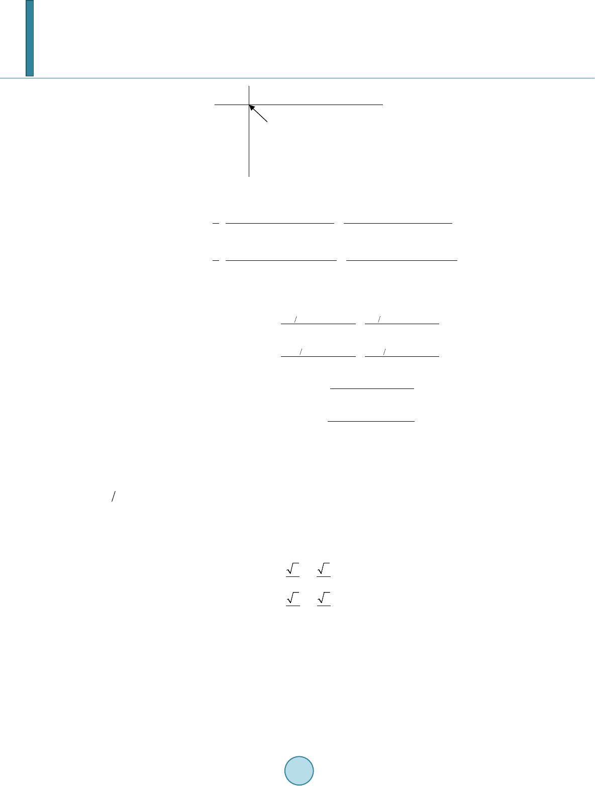 Y. Zhuang Figure 2. An intersection point of interface boundaries. ( ) 1, 11, 11, 11, 11, 11, 11, 11, 1 , 1 22 2 ij ijij ijij ijij ij xij cu cucu cu cu hh ++ ++−+−++− +−−−−− −− + = (6) ( ) 1, 11, 11, 11, 11, 11, 11,11, 1 , 1 22 2 ijij ijijijij ijij yij du dudu du du hh ++ +++− +−−+ −+−−−− −− + ≈ (7) If is not an intersecting point of interface boundaries, the conventional central finite difference is use to approximate the right hand of Equation (4), i.e., is approximated by 1 2,1,,1 2,,1, 22 ( )( ) ijij ijijijij auu auu hh ++− − −− − , (8) is approximated by ,12 ,1,,12,,1 22 ( )( ) ij ij ijijijij auua uu hh ++− − −− − , (9) is approximated by 1, 1,1, 1, 2 i ji ji ji j cu cu h ++ −− − , (10) is approximated by ,1,1 ,1,1 2 ij ijij ij du du h ++ −− − . (11) It is known that central finite difference schemes (10) and (11) have second-order accuracy with er- rors. It is also easy to verify using Taylor expansion that schemes (6) and (7) have second-order accuracy. Also, comparing schemes (6) and (10), one can see that scheme (6) is the average of scheme (10) used at the two grid points and , and then the second order accuracy of scheme (6) follows from the fact that ( ) ( ) 3 11 12 j jj ff fOh −+ = ++ for any smooth function . Scheme (5) also has second-order accuracy. To see that, one can verify that ( ) ( ) ( )( ) ( ) ( ) ,(,),( ,) xy ywvv xv axyuaxyuawv uawvu+=+ (12) under the change of variables 22 22 22 22 x wv y wv = − = + (13) With Equality (12) under the change of variables (13), one can easily prove that scheme (5) has second-order accuracy. Actually, Scheme (5) is the application of schemes (8) and (9) along the two new variables and , which are actually representing the two diagonal lines and in the original coordinate space of variables and . These discussions show that the new finite difference schemes (5-7) have second-order accuracy, which is stated in the following Theorem. Theorem. Finite difference schemes (5-7) for approximating the differential operators on the right hand side of Equation (4) at intersecting point of interface boundaries have second-order accuracy with errors of order . 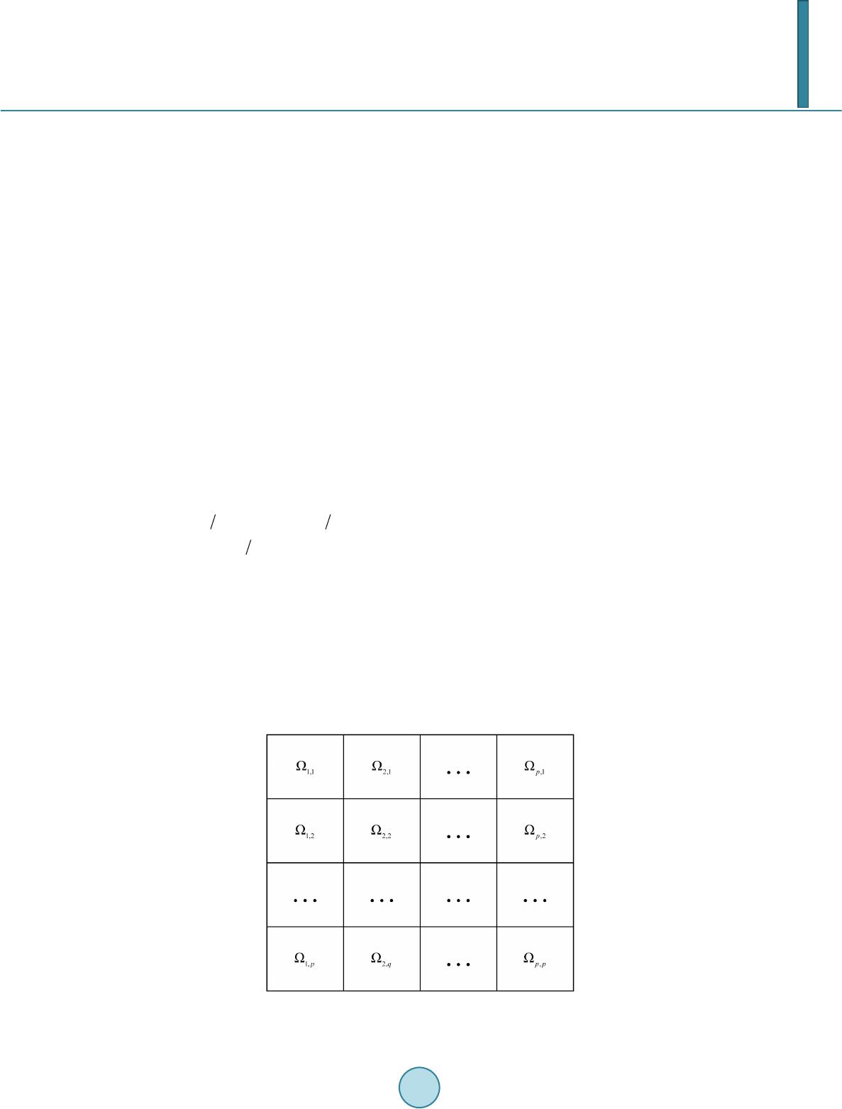 Y. Zhuang The theorem above means that finite different Schemes (5 - 7) have good accuracy, as good as the conve n- tional schemes (8 - 11). Now, let us look at another feature of Schemes (5 - 7) in term of its impact on the SEIDD methods. From the formulas of schemes (5-7), one can see that the solution is used at points , , , , and is to approximate the right hand side of Equation (4). Since is an intersecting point of interface boundaries, points , , , and are in subdomains. So for the stabilization step of the SEIDD method, i.e . Step 3 of the SEIDD me- thod, Schemes (5-7) use the solution at points , , , and are , , , and , components of the solution on the subdomains which have been computed in Step 2. But Schemes (5-7) do not use the solution on any point on the interface boundaries except point . Thus, the discrete equation of the stabilization step of a SEIDD method that involves solution at point does not involve any other grid points on the interface boundaries, leading to the decoupling of discrete equation on an intersecting point of interface boundaries from all other discrete equations on other interface boundaries. Such decoupling enables the efficient parallel processing of the solution process without all-to-all communica- tions for the stabilization step. In addition to decoupling the discrete equations on interface boundaries, another feature of Schemes (5-7) is that the scheme is very simple to implement into simulation code and does not require sophisticated program- ming techniques, which is very helpful for simulation code development and hence lower the chance of code bugs due to its code implementation simplicity. 4. Numerical Experiments To experimentally examine the performance of finite difference schemes (5-7), we choose two testing problems on the same spatial domain square domain . The two problems are 1. () [(112cos )][112cos](11.5cos ) t xxyy uxux uxu = ++ +++ with solution ; 2. ( ) y u12sin2(cos)(3-2 cos22 sin) txx yyx uuxuyuxy u+++ += + with solution . Uniform spatial grid of was chosen so that the x-direction and y-direction mesh size is . The simulation time interval is and the total simulation time steps is 4000 with a time step size . To test the proposed finite difference schemes (5-7), the spatial domain is divided into equal-size square sub-subdomains as in Figure 3, with ranging from 1 to 256, and each square sub -subdomain is assigned to a different processor. On intersecting points of interface boundaries, Schemes (5-7) was used to discretize the equation. On other points, including points in subdomains and on interface boundaries, standard finite difference schemes (8-11) were used. With the spatial discretization, the equation on each subdomain is solved by a modified symmetric successive over-relaxation (QSSOR) tailore d to non-symm etric matrices [40] with 30 QSSOR iterations. The Figure 3. Illustration of the domain partition. 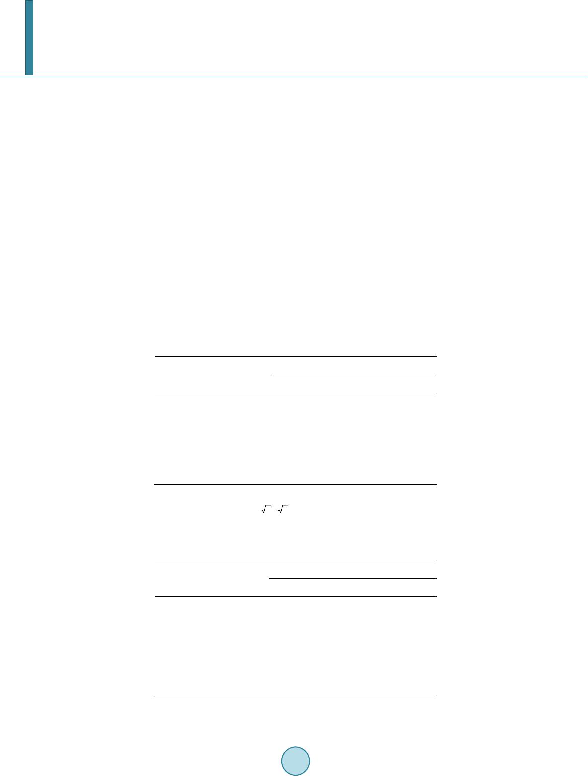 Y. Zhuang equations on the interface boundaries in Step 3 (except equations at the intersecting points) are tridiagonal sys- tems and are solved by a tridiagonal solver. The computation on Step 1 is a matrix-vector multiplication since it uses the forward Euler method. We measured the errors of the computed solution in ∞-norm, i.e. the maximum errors at time t = 1, and listed the errors in Table 1 for the two problems for the indicated number of subdo- mai ns. To compare the result of using Schemes (5-7) with the result of using the conventional central finite differ- ence, we also used schemes (8-11) for discretizing Equation (4). Since using Schemes (8-11) would couple all grid points on the interface boundaries together into a discrete equation on all interface boundary points, the domain is partitioned as in Figure 1(b) or Fig ure 1(c) with no intersecting points of interface boundaries. We measured the errors of the computed solution in ∞-norm at time t = 1, and listed the errors in Table 2 for the two problems for the indicated number of subdomains. The test data show that when the number of subdomains reaches 64 or larger, the new finite difference scheme produces higher accuracy. 5. Concluding Remarks Stabilized explicit-implicit domain decomposition provides efficient, stable, and highly parallel methods for solving time-dependent partial difference equations of the parabolic type on parallel computers, but suffer from a restriction that the interface boundaries must not intersect inside the domain. In this paper, we present a finite difference scheme for discretizing the equation spatially, which is of high simplicity, easy to implement, attains second-order spatial discretization accuracy as does the conventional central finite difference, and allows inter- face boundaries to intersect inside the domain. Table 1. Maximum errors with the new finite difference scheme. P m n 1melborP 2melborP Max-err Max-err 1 2048 × 2048 4.616e−05 7.164e−05 4 1024 × 1024 4.616e−05 5.629e−05 16 512 × 512 2.430e−05 5.629e−05 64 256 × 256 9.942e−06 1.373e−05 256 128 × 128 3.275e−05 4.437e−05 The domain is with h = 2π/2048, and the time interval is [0,1] with 1/4000. The domain divided into equal-size subdomains, where is the num- ber of processors. The second column under m × n indicates the discrete grid size of each subdomain. When P = 1, there is Scheme 5 is not used since there is no interface boundary. Table 2. Maximum errors with the standard finite difference P m × n 1melborP 2melborP Max-err Max-err 1 2048 × 2048 4.616e−05 7.164e−05 4 512 × 2048 3.483e−05 7.163e−05 16 128 × 2048 9.676e−06 1.396e−05 64 32 × 2048 1.103e−04 1.591e−04 256 8 × 2048 5.780e−04 8.516e−04 Note that when P = 1, the method and the data are exactly same as those in Table 1 since no interface boundaries.  Y. Zhuang Acknowledgements The numerical tests were carried out on systems managed by the Texas Tech High Performance Computing Center. Their help is acknowl ed ged. References [1] Bogetti, T.A. and Gillespie, J.A. (1991) Two-Dimensional Cure Simulation of Thick Thermosetting Composites. Journal of Composite Materials, 25, 239-273. [2] Myers, P.S., Uyehara, O.A. and Borman, G.L. (1967) Fundamentals of Heat Flow in Welding. Welding Research Council Bulletin, 123. [3] Stubblefield, M., Yang, C., Lea, R. and Pang, S. (1998) The Development of Heat-Activated Joining Technology for Composite-to-Composite Pipe Using Prepreg Fabric. Polymer Engineering and Science, 38, 143-149. [4] Cogger, C.G., Hajjar, L.M., Moe, C.L. and Sobsey, M.D. (1988) Septic System Performance on a Coastal Barrier Isl- and. Journal of Environmental Quality, 17, 401 -408. [5] Hagedorn, C., Han sen , D.T. and Simonson, G.H. (1978) Survival and Movement of Fecal Indicator Bacteria in Soil under Conditions of Saturated Flow. Journal of Environmental Quality, 7, 55-59. [6] Sportisse, B. and Djouad, A. (2000) Reduction of Chemical Kinetics in Air Pollution Modeling. Journal of Computa- tional Physics, 164 , 354 -376. http://dx.doi.org/10.1006/jcph.2000.6601 [7] Bowe r , J.M. and Beeman, D. (199 8) The Book of GENESIS: Exploring Realistic Neural Models with the General NEural SImulation System. 2nd Edition, Springer Verlag, New York. http://dx.doi.org/10.10 07 /978 -1-4612-1634-6 [8] Dayan, P. and Abbott, L.F. (2001) Theoretical Neuroscience: Computational and Mathematical Modeling of Neural Systems. The MIT Press, Cambridge. [9] Koch, C. (1999) Biophysics of Computation: Information Processing in Single Neurons. Oxford University Press, New York. [10] Zhuang, Y. (2006) A Parallel and Efficient Algorithm for Multi-Compartment Neuronal Modeling. Neurocomputing, 69, 1035-1038. [11] The Nobel Foundation, The Nobel Prize in Physiology or Medicine 1998. Nobelprize. org. http://nobelprize.org/nobel_prizes/medicine/laureates/1998/illpres/ [12] Philippides, A., Husbands, P., Smith, T. and O’Shea, M. (2004) Structure-Based Models of NO Diffusion in the Nerv- ous System. In: Feng, J., Ed., Computational Neuroscience: A Comprehensive Approach, Chapman & Hall/CRC, London, 97-130. [13] Black, K. (1992) Polynomial Collocation Using a Domain Decomposition Solution to Parabolic PDE’s via the Penalty Method and Explicit-Implicit Time Marching. Journal of Scientific Computing, 7, 313-338. http://dx.doi.org/10.1007/BF01108035 [14] Chen , H. and Lazarov, R. (19 96 ) Domain Splitting Algorithm for Mixed Finite Element Approximations to Parabolic Problems. East-West Journal of Numerical Mathematics, 4, 121-135. [15] Daoud, D.S., K h al iq , A.Q.M. and Wade, B.A. (2000) A Non-Overlapping Implicit Predictor-Corrector Scheme for Pa- rabolic Equations, Proceeding of International Conf. Parallel & Distributed Processing Techniques & Applications (PDPTA 2000) Las Vegas, NV, H.R Arabnia et al., ed., Vol. 1, CSREA Press, 15-19. [16] Dawson, C. and Dupont, T. (1994 ) Explicit/Implicit, Conservative Domain Decomposition Procedures for Parabolic Problems Based on Bloc k-Centered Finite Difference. SIAM Journal on Numerical Analysis, 31, 1045-10 61 . [17] Dawson, C., Du, Q. and Dupont, T. (1991) A finite Difference Domain Decomposition Algorithm for Numerical Solu- tion of the Heat Equation, Mathematics of Computation, 57, 63-71. [18] Dryja , M. and Tu , X. (2007) A Domain Decomposition Discretization of Parabolic Problems. Numerische Mathematik, 107, 625-640. http://dx.doi.org/10.1007/s00211-007-0103-0 [19] Du, Q., Mu, M. and Wu, Z.N. (2001) Efficient Parallel algorithMs for Parabolic Problems. SIAM Journal on Numerical Analysis, 39, 1469 -1487 . http://dx.doi.org/10.1137/S0036142900381710 [20] Jun, Y. and Mai, T.-Z. (2006) ADI Meth od -D omain Decomposition. Applied Numerical Mathematics, 56, 1092-1107 . http://dx.doi.org/10.1016/j.apnum.2005.09.008 [21] Kuznetsov, Y.A. (1988) New Algorithms for Approximate Realization of Implicit Difference Schemes. Sov. J. Numner. Ana. Math. Modell., 3, 99-114. [22] Kuznetsov, Y.A. (1990) Domain Decomposition Methods for Unsteady Convection-Diffusion Pr o blems . Proc. of the 9th Int. Conf. Computing Methods in Applied Sciences and Engineering, Paris, 29 Jan uary-2 Feb ruary1990, 211-227. 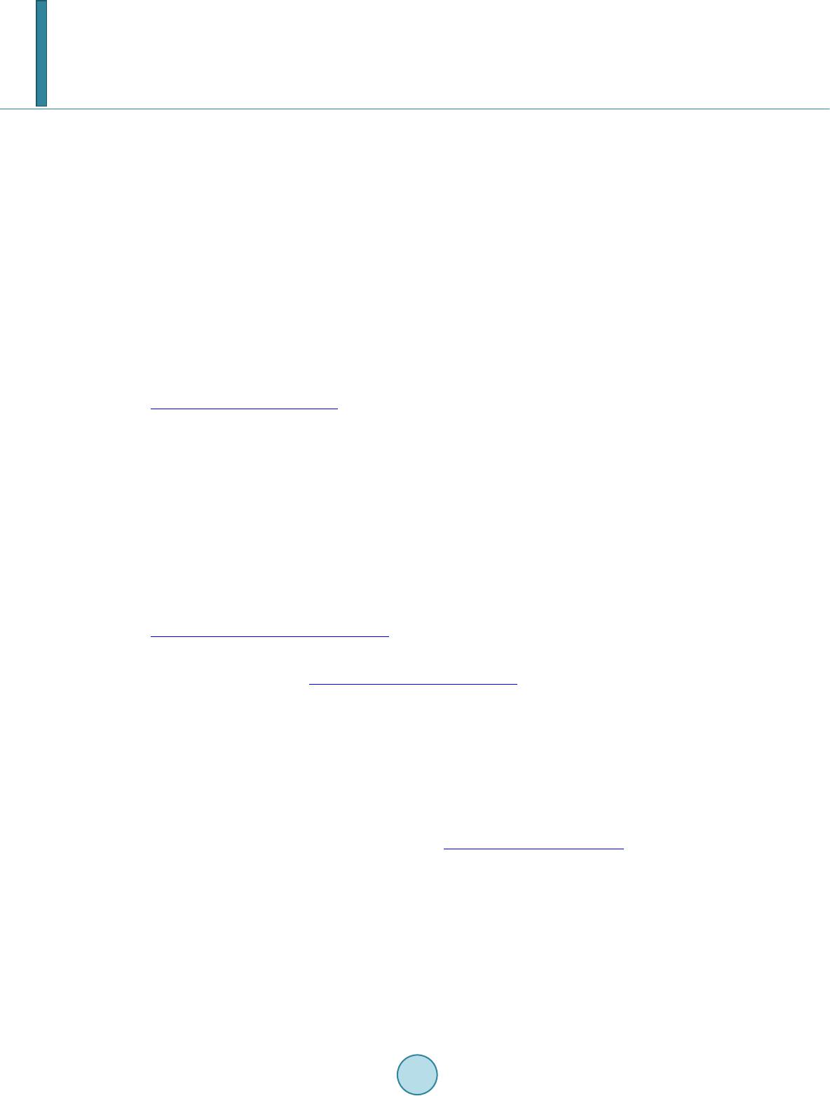 Y. Zhuang [23] Lae vsk y, Y.M. (1992) A Domain Decomposition Algorithm without Overlapping Subdomains for the Solution of Pa- rabolic Equations (Russian). Zh. Vychisl. Mat. i Mat. Fiz., 32, 1 744 -17 55; Translation in Computational Mathematics and Mathematical Physics, 32, 1569-1580. [24] Lae vsk y, Y.M. (1993) Explicit Implicit Domain Decomposition Method for Solving Parabolic Equations, Computing Methods and Technology for Solving Problems in Mathematical Physics (Russian) 30-46, Ross. Akad. Nauk Sibirsk. Otdel., Vychisl. Tsentr, Novosibirsk. [25] Lae vs ky, Y.M. and Gololobov, S.V. (1995) Explicit-Implicit Domain Decomposition Methods for the Solution of Pa- rabolic Equations. (Russian) Sibirsk. Mat. Zh., 36, 590-601, ii; Translation in Siberian Math. J., 36, 506 -516. [26] Lae vsk y, Y.M. and Rudenko, O.V. (19 95 ) Splitting Methods for Parabolic Problems in Nonrectangular Domains. Ap- plied Mathematics Letters, 8, 9-14. [27] Lia o , H. L. , Shi, H.S. and Sun, Z.Z. (2009) Corrected Explicit-Implicit Domain Decomposition Algorithms for Two-Di- mensional Semilinear Parabolic Equations. Science in China, Series A: Mathematics, 52, 2362-2388. [28] Qian , H. and Zhu, J. (1998) On an Efficient Parallel Algorithm for Solving Time Dependent Partial differential Equa- tions. Proceedings of the 11th International Conference on Parallel and Distributed Processing Techniques and Ap- plications, Las Vegas, CSREA Press, Athens, 394-401. [29] Shi, H.S. and Liao, H.L. (2006) Unconditional Stability of Corrected Explicit-Implicit Domain Decomposition Algo- rithms for Parallel Approximation of Heat Equations. SIAM Journal on Numerical Analysis, 44, 1584-1611. http://dx.doi.org/10.1137/040609215 [30] Zhu, L., Yuan, G. and Du, Q. (2009) An Explicit-Implicit Predictor-Corrector Domain Decomposition Method for Time Dependent Multi-Dimensional Convection Diffusion Equations. Numerical Mathematics: Theory, Methods and Applications, 2, 1-25. [31] Zhu, L. , Yuan, G. and Du, Q. (2010) An Efficient Explicit/Implicit Domain Decomposition Method for Convec- tion-Diffusion Equations. Numerical Methods for Partial Differential Equations, 26, 852-873. [32] Zhuang, Y. and Sun, X.-H. (1999) A Domain Decomposition Based Parallel Solver for Time Dependent Differential Equations. Proc. 9th SIAM Conf. Parallel Processing for Scientific Computing, March 1999, San Antonio, Texas. CD-ROM SIAM, Philadelphia, 1999. [33] Zhuang, Y. and Sun, X.-H. (2001) Stable, Globally Non-Iterative, Non -Overlapping Domain Decomposition Parallel Solvers for Parabolic Problems. Proceedings of ACM/IEEE Super Computing Conference, Denver, Colorado, Novem- ber 2001. CD-ROM IEEE Computer Society and ACM. [34] Zhuang Y. and Sun, X.-H. (20 02) Stabilized Explicit Implicit Domain Decomposition Methods for the Numerical So- lution of Parabolic Equations. SIAM: SIAM Journal on Scientific Computing, 24, 335-358. http://dx.doi.org/10.1137/S1064827501384755 [35] Zhuang Y. and Sun, X.-H. (2005) A Highly Parallel Algorithm for the Numerical Simulation of Unsteady Diffusion Processes . Proceedings of the 19th IEEE International Parallel and Distributed Processing Symposium (IPDP S ), Denver, Colorado, April 2005. http://dx.doi.org/10.1109/IPDPS.2005.32 [36] Zhuang, Y. (2007) An Alternating Explicit Implicit Domain Decomposition Method for the Parallel Solution of P ara- bolic Equations. Journal of Computational and Applied Mathematics, 206, 549-566. [37] Wan g, J., Wu, H. and Zhuang, Y. (2011) A Parallel Domain Decomposition Algorithm for Solving the Equation of Ni- tric Oxide Diffusion in the Nervous System. Proc. International Conf. Parallel & Distributed Processing Techniques & Applications (PDPTA ’11) Las Vegas, Nevada. [38] Zhuang, Y. and Wu, H. (2012 ) Efficient Parabolic Solvers Scalable Across Multi-Architectural Levels. Pro c. 10th IEEE International Symposium on Parallel & Distributed Processing with Applications (I S PA ), Leganés, Madrid, 10-13 July 2012. [39] Jun, Y. and Mai, T.-Z. (2009) Numerical Analysis of the Rectangular Domain Decomposition Method. Communica- tions in Numerical Methods in Engineering, 25, 810 -826. http://dx.doi.org/10.1002/cnm.1158 [40] Zhuang, Y. (2005 ) Quasi-Symmetric Successive Over-Relaxation for Non -Symmetric Linear Systems, Preprint.
|