Circuits and Systems
Vol.07 No.10(2016), Article ID:70154,11 pages
10.4236/cs.2016.710285
A Multi-Hop Dynamic Path-Selection (MHDP) Algorithm for the Augmented Lifetime of Wireless Sensor Networks
Perumal Kalyanasundaram1, Thangavel Gnanasekaran2
1Department of Electronics and Communication Engineering, Nandha Engineering College, Erode, India
2Department of Information Technology, RMK Engineering College, Chennai, India

Copyright © 2016 by authors and Scientific Research Publishing Inc.
This work is licensed under the Creative Commons Attribution International License (CC BY).
http://creativecommons.org/licenses/by/4.0/


Received 3 May 2016; accepted 15 May 2016; published 29 August 2016
ABSTRACT
In Wireless Sensor Networks (WSN), the lifetime of sensors is the crucial issue. Numerous schemes are proposed to augment the life time of sensors based on the wide range of parameters. In majority of the cases, the center of attraction will be the nodes’ lifetime enhancement and routing. In the scenario of cluster based WSN, multi-hop mode of communication reduces the communication cast by increasing average delay and also increases the routing overhead. In this proposed scheme, two ideas are introduced to overcome the delay and routing overhead. To achieve the higher degree in the lifetime of the nodes, the residual energy (remaining energy) of the nodes for multi-hop node choice is taken into consideration first. Then the modification in the routing protocol is evolved (Multi-Hop Dynamic Path-Selection Algorithm―MHDP). A dynamic path updating is initiated in frequent interval based on nodes residual energy to avoid the data loss due to path extrication and also to avoid the early dying of nodes due to elevation of data forwarding. The proposed method improves network’s lifetime significantly. The diminution in the average delay and increment in the lifetime of network are also accomplished. The MHDP offers 50% delay lesser than clustering. The average residual energy is 20% higher than clustering and 10% higher than multi-hop clustering. The proposed method improves network lifetime by 40% than clustering and 30% than multi-hop clustering which is considerably much better than the preceding methods.
Keywords:
Wireless Sensor Networks (WSN), Cluster Based WSN, Multi-Hop Mode, Residual Energy, Average Delay, Multi-Hop Dynamic Path-Selection Algorithm, Life Time

1. Introduction
Wireless Sensor Network is principally composed of a base station and several sensor nodes scattered over a finite geographical area. The nodes supervise the environment in which they are installed to gather information such as humidity, temperature, pressure, sound, vibration and so on. Every node in the WSN relays the information. It is congregated to the Base Station (BS) directly or through multi-hop wireless communication link.
A wireless sensor node comprises of four major components: a sensing unit to observe the environment; a processing unit to process the information; a radio transceiver unit for the sharing of the gathered data; power supply unit.
Naturally, sensor nodes are energy embarrassed, since they rely on batteries as energy source. The sensors are consuming the power from the battery when they are operative. Due to energy constrictions, the lifetime of a WSN is also limited. The battery replacement in the nodes is cumbersome process [1] . Therefore, to diminish the energy consumption in each node and to prolong the lifetime of the sensors in a network, various schemes are proposed to augment the lifetime of sensors based on the wide range of parameters. In majority of the cases, the center of attraction will be the nodes’ lifetime enhancement and routing. In the scenario of cluster based WSN [2] , multi-hop mode of communication with Low Energy Adaptive Clustering Hierarchy (LEACH) reduces the communication cast by increasing average delay and also increases the routing overhead. The inspiration behind this effort is to decrease the energy consumption of the sensor nodes by increasing the clustering hierarchy.
In WSNs, the information about the amount of residual energy found dispersed in the network is called an energy map. By judging the available amount of residual energy in each part of the network, corrective measures can be taken by redeploying additional nodes before any part of the network gets disjointed due to energy depletion [3] . Modified routing protocols can also use the information offered by an energy map to reroute the traffic through the nodes with privileged residual energy, so that nodes with a reduced amount of residual energy can conserve their energy for future use.
Managing power consumption in wireless sensor network from low level node architecture to high level communication protocols is a tedious task. A more appropriate approach is the construction of residual energy distribution map towards the networks energy consumption behavior.
The remaining part of this paper is organized as follows. Section 2 converses related work. Section 3 introduces the problem formulation. Section 4 outlines the proposed work. Section 5 elaborates Multi-Hop Dynamic Path-selection (MHDP) algorithm. Section 6 depicts performance evaluation and analysis. Finally, Section 7 concludes the paper.
2. Related Works
There are several necessities for a clustering algorithm. A centralized controlled mechanism is not practical in a large-scale sensor network. All the sensor nodes should be well connected to the cluster heads in such a way to make energy consumption be well-balanced among all sensor nodes [4] . Third, the energy efficient clustering algorithm is mandatory to improve the life time of network. In practical, it is inflexible to ensure the same battery capacity in all nodes [5] . The amount of the energy consumed differs in gathering data among cluster heads, and it reflects on the number of cluster members and their locality. The consumption of Energy varies among the cluster members due to the unusual distances to a cluster-head. Additionally, redeployment for prolonging network lifetime will also be the major cause of the inconsistent residual energy among all sensor nodes. LEACH’s clustering algorithm [6] presumes that sensor nodes are homogenous and equally powered. However, in practical, it is an ideal case. LEACH cannot accommodate the changes in sensor networks as the addition, removal of the sensor nodes. Finally, the cluster head have to broadcast its own advertisement to the entire sensor network in cluster formation phase of LEACH, which will cause another inefficient use of energy [7] .
Energy Efficient Cluster Selection elects cluster heads in such a way that they should be the nodes with more residual energy with no iteration and a good cluster head distribution is achieved. In many clustering algorithms in wireless sensor networks, the residual energy is considered to prolong the sensor network lifetime.
For instance, as shown in Figure 1, let us consider a sensor network deployed with seven nodes. Nodes D and C are located in each other’s cluster range and the amount of the residual energy of node D and node C is higher than that of the other sensor nodes. Cluster selection is carried out based on its residual energy. Apparently, selection of the node C as a cluster head is the highest probability. As a result, there is a least probability of the

Figure 1. A sensor network deployed with seven nodes.
other nodes with lower residual energy to be selected as a cluster head. As a cluster head deals with large number of member nodes, it consumes more energy than a plain node. The energy of nodes within the cluster range of node D will be drained rapidly.
After clustering, all the cluster heads broadcast the Weight message within a range having the radius R, which contains weight W and node ID. The cluster head judges against its own weight with the weight contained in the Weight message expected from its neighbor cluster head. If it has less significant weight, it selects the node that has the biggest weight as its parents and confirms with the CHILD message to the parent node. Finally, after a precise time, a routing tree will be framed. After routing tree formation, a TDMA schedule is broadcasted by the cluster heads to their active member nodes.
In Figure 2, nodes A to E are cluster heads with their weights specified in parenthesis. The node B will get a WEIGHT message from A, C, D, E and node A is selected as its parent. In the same way, node D and E select node B as their parent, and node C opts node A as its parent. Node A obtains a WEIGHT message from nodes C and B, but due to their less weight than node A, A will be the root node that establishes the communication with the base station and routing tree is built.
The weight W of node i is defined as:
 (1)
(1)
where RSSi denotes the received signal strength of node i for the signal broadcasted by the base station, RSSmax is a constant which is decided by the deployment of the base station, and the function D is the estimation of the distance between node i and the Base Station (BS). After the installation of sensors, the base station broadcasts the probing message to all sensor nodes and they obtain the RSS according to the received signal strength. RSS will be constant during the network lifetime until base station varies its location or sensor nodes are moving. Due to its higher weight, the node which is closer to the base station and finds in a sub region with full energy will be the root node of routing tree.
Once a node becomes a cluster head then it starts to broadcast advertisement (ADV) message. Upon reception of this advertisement ADV message, every non cluster node will make a decision to join a certain Cluster Head (CH) based on the Received Signal Strength (RSS). A TDMA based transmission schedule is created by CH for each node in the cluster. CH cumulates the data received from multiple nodes and forwards it to the base station. This communication protocol employs in various rounds and a different sensor node is selected as a cluster head based on the following formula in order to compensate the load among all participating nodes [8] .
The threshold is set as:
 (2)
(2)

Figure 2. Routing tree construction.
where, “P” be the required percentage of cluster heads (e.g., P = 0:05), “r” be the current round, and “G” be the set of nodes which have not been cluster-heads in the previous 1/P rounds. With this threshold, we observe that each node will be a Cluster Head (CH) at some point within 1/P rounds. During 0th round (r = 0), each sensor node has a probability P to become a cluster-head. The nodes that are become CH during round 0 cannot be CH for the next 1/P rounds. Therefore the probability that the remaining nodes to become cluster heads is increased, since there are few nodes that are entitled to become cluster-heads. At the end of (1/P)-1 rounds, T = 1 for any sensor node that have not yet been CH, and after 1/P rounds, all sensor nodes are eligible to become CH. The number is a lesser amount than the threshold T(n), the node will become a cluster-head for the current round.
To reduce the energy consumption wireless sensor networks adopt clustering at multiple levels few protocols establish couple of clustering levels while others trying to make use of the resources efficiently by multi-hop routing with unequal clustering [9] [10] . It is depicted in Figure 3.
1) If clustering is done at fewer levels, cluster heads are in a position to transmit data with higher power to reach other cluster heads or the base station.
2) As the selection of the cluster head is carried out done by the member nodes, cluster head which is very near to base station will act as cluster head for a bulk of lower level cluster heads. Therefore, nodes close to the base station will become short lived.
Another budding approach for the routing in WSN is multi-hop routing with unequal clustering. The intermediate nodes will try to forward data to the base station in this approach, based on the location of the sensed data.
A multi-hop routing algorithm for WSN with equal clustering will achieve the following objectives.
1) The network life time is extended by reducing the average distance of each Cluster Head (CH) from its upper level cluster head so that the consumption of energy is distributed among different cluster heads.
2) The base station will select the cluster heads at second and above which in turn reduces computational cost at sensor nodes.
3) As equal number of clustering level is used, global TDM schedule will be sufficient.
Figure 5 shows dissimilar existent routing schemes for wireless sensor networks.
Figure 4(a) depicts the state of single hop communication without clustering i.e., each sensor node forwards data directly to the Base Station. Figure 4(b) shows the multi-hop communication without clustering, That is, the intermediate sensor nodes sends data from source node to the Base Station. Figure 4(c) enumerates single hop clustering based communication i.e., member node broadcast to Cluster Head and Cluster Head broadcast data to Base Station. Figure 4(d) shows multi-hop routing environment with clustering.
After formation of the cluster heads at different levels, scheduling of member nodes needs to be carried out. Due to low energy consumption, Time Division Multiple Access (TDMA) is the ideal scheduling scheme in sensor networks. To guarantee data delivery in the communication between a cluster head and its upper cluster head, higher power is required. Upper level cluster heads will be allocated with longer time slots than their member low level cluster heads. Figure 5 shows the time slot issued by a cluster head having two Cluster Heads along with five simple member nodes. The Time slots T1 to T5 are assigned to upper level simple member nodes and time slots T6 and T7 are assigned to lower level member cluster heads.

Figure 3. Clustering in multi-hop transmission model.
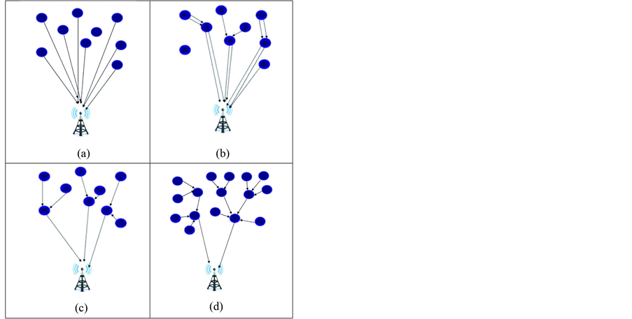
Figure 4. Different data forwarding scenario with and without clustering.

Figure 5. TDMA slot for member nodes.
3. Problem Formulation
In this section, we will formulate few assumptions about the network model before problem statement. We assume that N sensor nodes are randomly deployed in a two-dimensional square field A, and the properties of the sensor network are assumed as mentioned below:
1) This network is a densely deployed static network. It defines a large number of sensor nodes are closely deployed in a two-dimensional geographic area and the nodes do not have the mobility after deployment.
2) The energy of sensor nodes cannot be recharged.
Numerous schemes are proposed to augment the life time of sensors based on the wide range of parameters. In majority of the cases, the center of attraction will be the nodes’ lifetime enhancement and routing. In the scenario of cluster based WSN, multi-hop mode of communication reduces the communication cast by increasing average delay and also increases the routing overhead. In this proposed scheme, two ideas are introduced to overcome the delay and routing overhead. To achieve the higher degree in the lifetime of the nodes, residual energy (remaining energy) of the nodes for multi-hop node choice is taken into consideration first. Then the modification in the routing protocol is evolved. A dynamic path updating is initiated in frequent interval based on nodes residual energy to avoid the data loss due to path extrication and also to avoid the early dying of nodes due to elevation of data forwarding [11] . The proposed method improves network lifetime considerably much better than the preceding methods.
4. Proposed Work
The proposed task is achieved by executing the following three phases
In the first stage, initialization of Sensor nodes is taken place. In this scenario, Self-configurable nodes update their information each other. Next stage involves Cluster construction and CH election. Grouping of nodes and election for CH is carried out by broadcast advertise [12] and join or response messages. CH nodes collect the data’s from the node and forward it to base station either single hop or multi hop depending on their connectivity fashion.
The Sync () process is invoked when members of two clusters meet and both members pass the membership check. It is designed to share and synchronize the two local tables. The synchronization process is mandatory because each node separately learns network parameters, which may vary from one node to another node. The Time Stamp field is utilized for the “better” awareness of the network to deal with any clash. The Lower stability node must leave the cluster. The node stability is defined to be its minimum probability of contact with in the cluster members. It indicates the likelihood that the node will be excluded from the cluster due to the probability of low contact. The leaving node then clears its gateway table completely and reset its Cluster ID. The above task is accomplished by Leave () procedure. The Join () procedure is employed for a node to join a “better” cluster or to merge two separate clusters.
Data forwarding is accomplished with the proposed Multi-Hop Dynamic Path-selection (MHDP) Algorithm. If a Cluster Head X, finds the base within the critical distance d0 then it chooses the single hop to reach base station, otherwise the choice is the multi-hop with modified routing algorithm [13] .
This proposed system (Figure 6) employed in various rounds and a different node is selected as a cluster head based on the following formula in order to compensate the load among all participating nodes by considering the residual energy.
5. Multi-Hop Dynamic Path-Selection (MHDP) Algorithm
In this proposed algorithm, two ideas are commenced to conquer the delay and routing overhead. To achieve the higher degree in the lifetime of WSN, the residual energy the nodes for multi-hop node choice is taken into account. Then the modification in the routing protocol is developed. A dynamic path updating is initiated infrequent interval based on nodes residual energy to avoid the data loss due to path extrication and also to avoid the early dying of nodes due to elevation of data forwarding. This course of action is carried out in the following steps. Figure 7 depicts the three steps.
Step 1: Construction of Neighboring Graph
Each sensor broadcasts its node id and location to their neighbors.
Each Node “n” prepares a list B(n) with node ids and locations as received from broadcast message.
Let A(n) be the adjacent nodes list for n, consists of all nodes, such that 
Step 2: Construction of Path set G(p)
Let i and j, be the sensor nodes in B(n).
Run the Bellman-Ford shortest path algorithm to determine a shortest path P(i, j), in the local neighboring graph, from “i” to j.
Bellman-Ford algorithm is used to find all shortest path in a graph from one source to all further nodes. It requires that the graph does not contain any cycles of negative length, but if it does, it is able to detect it. This

Figure 6. Flow chart for cluster formation and routing using MHDP.
algorithm is based on the relaxation procedure. This procedure considers two nodes as augments and an edge which connects these nodes.
Step 3: Binary Search tree for best path [14] .
Identify Maximum residual energy nodes in route.
Do a binary search in B(n) to find the maximum value max residual energy nodes. In this case there is a path “P” from source to destination that uses at reduced communication cast.
For this, when testing a path p, we find a shortest source to destination path that does not use node with minimum residual energy that build the residual energy fraction at “u” less than the threshold “q”.
Update the path details in path-set G(p).
Refresh this process in frequent interval.
To find the minimum value of the residual energy of the threshold will be calculate from the following formulae
 (3)
(3)

Figure 7. Flow chart for Multi-hop dynamic path-selection (MHDP) algorithm.
where  the residual energy of the node n is,
  is the average energy,
  is the maximum energy.
6. Performance Evaluation and Analysis
In the simulation experiments, network lifetime has been taken into consideration. The simulation is carried out for Clustering Method, Multi-hop transmission and the projected Multi-Hop Dynamic Path-selection (MHDP) algorithm. We choose some evaluation metrics to quantify the performance of Multi-Hop Dynamic Path-selec- tion (MHDP) algorithm are Average residual Energy, Average delay, Network Lifetime. The parameters of simulations are listed in Table 1. In the node deployment scenario, sensor nodes are assumed to be randomly deployed in are rectangular area of size 1500 m × 200 m. A total of 100 numbers of nodes are taken into account. The size of the data packet is predetermined as 500 bits. The initial energy of the nodes is assumed to be 1 J. With the predefined parameters, the simulation is carried out. Based on the results acquired from the simulation, analysis is instigated.
Figure 8 shows the relationship between the number of rounds and the average residual energy for Clustering, Multi-hop Clustering and Multi-hop Dynamic Path-selection (MHDP) algorithm. When the data transmission by the nodes is in progress, the power consumed by them is also high. This will make an impact on the residual energy of the nodes which are involved in data transmission.
We observe that by adopting the Multi-hop Dynamic Path-selection (MHDP) algorithm, the average residual energy of the nodes is 700 J which is higher than Clustering (500 J) and Multi-hop Clustering (600 J) during the 200th round. Obviously, our algorithm can work well even for the higher rounds. If Clustering is adopted almost 50% of the average residual energy is available after certain time period. By the adoption of Multi-hop clustering, 60% of average residual energy is obtainable. As the number of round increases, it can be seen that

Table 1. Simulation parameters.

Figure 8. Comparative analysis for average residual energy.
the performance of Multi-Hop Dynamic Path-selection (MHDP) algorithm is superior to the Clustering, Multi- hop Clustering by offering 70% of average residual energy.
Figure 9 shows the relationship between the number of rounds and the average delay experienced in Clustering, Multi-hop Clustering and Multi-Hop Dynamic Path-selection (MHDP) algorithm. The delay is the time difference between the starting of data transmission by the transmitter to the successful reception of the data by the receiver. Actually a time stamp is generated during the start of transmission and the time at which the data is received by the receiver successfully is noted. This time difference will point out the delay in transmission. The average value is calculated from the entire transmissions. This parameter may vary depending upon the number of nodes. The delay augments, if the number of nodes which are involved in data transmission increases. Therefore the fixed number of nodes is considered in this analysis. In the earlier rounds, the delay in the three methods is almost the same. If the round increases, the Clustering offers higher degree of delay. The clustering formation and communication with the Cluster head may introduce significant delay. By implementing Multi-hop the delay involved in the communication is reduced a minute level. Here the Clustering mechanism is abolished. However, the delay is at significant level, due to no adaption of dynamic path selection. As Multi-Hop Dynamic Path-selection (MHDP) algorithm offers higher degree of path selection by considering dynamic path selection which in turn diminish the average delay significantly.
We observe that by adopting the Multi-Hop Dynamic Path-selection (MHDP) algorithm the average delay is 0.88 ms which is significantly lower than Clustering (1.65 ms) and Multi-hop Clustering (1.43 ms) during the 200th round. Obviously, our algorithm can work well even for the higher rounds. Multi-hop Clustering offers almost 80% of the delay offered by Clustering. Multi-hop Dynamic Path-selection (MHDP) algorithm does only 50% of the delay experienced in Clustering.
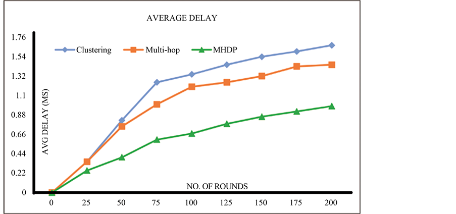
Figure 9. Comparative analysis for average delay.

Figure 10. Comparative analysis for number of alive nodes.
As the number of round increases, it can be noticed that the average delay of Multi-Hop Dynamic Path-selec- tion (MHDP) algorithm is much lesser than the Clustering, Multi-hop Clustering.
Figure 10 shows the relationship between the number of rounds and the number of alive nodes in Clustering, Multi-hop Clustering and Multi-hop Dynamic Path-selection (MHDP) algorithm. All the sensor nodes are battery powered intelligent nodes. During a course of time, the power level of the sensors goes down. The lifetime of network is defined by the period over which the power is derived from the power source. The lifetime of the sensors are varying depending on their individual functionality. In this analysis, it is observed that in earlier rounds the number of alive nodes during the process of Clustering, Multi-hop Clustering and Multi-hop Dynamic Path-selection (MHDP) are very close to each other, i.e. the number of died nodes are few in number. After a stipulated time period the number of alive nodes is drastically differing for different methods.
It is observed that by employing the Multi-hop Dynamic Path-selection (MHDP) algorithm the number of alive nodes is 30 which is appreciably higher than Clustering (0 nodes) and Multi-hop Clustering (0 nodes) during the 1400th round. Obviously, our algorithm can work sound even for the higher rounds. It is studied that Multi-hop Dynamic Path-selection (MHDP) algorithm is 40% efficient than Clustering and 30% efficient than Multi-hop Clustering. It is also viewed that Multi-hop Clustering is only 10% efficient than Clustering which is less significant than MHDP. As the number of round increases, it can be perceived that the number of alive nodes of Multi-Hop Dynamic Path-selection (MHDP) algorithm is higher than the Clustering, Multi-hop Clustering.
7. Conclusion
In this paper, we present Multi-Hop Dynamic Path-selection (MHDP) algorithm, a novel efficient algorithm. A dynamic path updating is initiated in frequent interval based on nodes residual energy to avoid the data loss due to path extrication and also to avoid the early dying of nodes due to elevation of data forwarding. The MHDP offers 50% delay lesser than Clustering. The average residual energy is 20% higher than Clustering and 10% higher than Multi-hop Clustering. The proposed method improves network lifetime by 40% than Clustering and 30% than Multi-hop Clustering which is considerably much better than the preceding methods. Simulation results confirm MHDP outperforms far better than Clustering and Multi-hop Clustering. In future work, the average residual energy achieved in this method can be further enhanced and average delay incurred can be further diminished by adopting suitable algorithms to achieve the augmented network lifetime.
Cite this paper
Perumal Kalyanasundaram,Thangavel Gnanasekaran, (2016) A Multi-Hop Dynamic Path-Selection (MHDP) Algorithm for the Augmented Lifetime of Wireless Sensor Networks. Circuits and Systems,07,3343-3353. doi: 10.4236/cs.2016.710285
References
- 1. Zhang, D.G., Li, G., Zheng, K., Ming, X.C. and Pan, Z.-H. (2014) An Energy-Balanced Routing Method Based on Forward-Aware Factor for Wireless Sensor Networks. IEEE Transactions on Industrial Informatics, 10, 766-773.
http://dx.doi.org/10.1109/TII.2013.2250910 - 2. Kumar, V., Jain, S. and Tiwari, S. (2011) Energy Efficient Clustering Algorithms in Wireless Sensor Networks: A Survey. IJCSI—International Journal of Computer Science Issues, 8, 259-268.
- 3. Mardini, W., Khamayseh, Y and Al-Eide, S. (2012) Optimal Number of Relays in Cooperative Communication in Wireless Sensor Networks. Communications and Network, 4, 101-110.
http://dx.doi.org/10.4236/cn.2012.42014 - 4. Lee, C. and Jeong, T. (2011) FRCA: A Fuzzy Relevance-Based Cluster Head Selection Algorithm for Wireless Mobile Ad-Hoc Sensor Networks. Sensors, 11, 5383-5401.
http://dx.doi.org/10.3390/s110505383 - 5. Thirumoorthy, P. and Karthikeyan, N.K. (2015) Secure and Effectual Energy Dynamic Routing Protocol for In-Net- work Aggregation in WSN. International Journal of Applied Engineering Research, 10, 6593-6597.
- 6. Xu, L.-L. and Zhang, J.-J. (2010) Improved LEACH Cluster Head Multi-hops Algorithm in Wireless Sensor Networks. 9th International Symposium on Distributed Computing and Applications to Business, Engineering and Science, Hong Kong, 10-12 August 2010, 263-267.
- 7. Liu, M., Cao, J.N., Chen, G.H. and Wang, X.M. (2009) An Energy-Aware Routing Protocol in Wireless Sensor Networks. Sensors, 9, 445-462.
http://dx.doi.org/10.3390/s90100445 - 8. Farooq, M.O., Dogar, A.B. and Shah, G.A. (2010) MR-LEACH: Multi-Hop Routing with Low Energy Adaptive Clustering Hierarchy. 2010 4th International Conference on Sensor Technologies and Applications, Venice, 18-25 July 2010, 262-268.
- 9. Yaacoub, E. and Abu-Dayya, A. (2012) Wireless Sensor Networks—Technology and Protocols. QU Wireless Innovations Center (QUWIC), Doha.
- 10. Vural, S. and Ekici, E. (2010) On Multihop Distances in Wireless Sensor Networks with Random Node Locations. IEEE Transactions on Mobile Computing, 9, 540-552.
http://dx.doi.org/10.1109/TMC.2009.151 - 11. Khan, A.W., Abdullah, A.H., Razzaque, M.A. and Bangash, J.I. (2015) VGDRA: A Virtual Grid-Based Dynamic Routes Adjustment Scheme for Mobile Sink-Based Wireless Sensor Networks. IEEE Sensors Journal, 15, 526-534.
http://dx.doi.org/10.1109/JSEN.2014.2347137 - 12. Nam, C.S., Han, Y.S. and Shin, D.R. (2011) Multi-Hop Routing-Based Optimization of the Number of Cluster-Heads in Wireless Sensor Networks. Sensors, 11, 2875-2884.
- 13. Thirumoorthy, P. and Karthikeyan, N.K. (2014) An Effectual Routing Protocol for In-Network Aggregation in Wireless Sensor Networks. Advances in Natural and Applied Sciences, 8, 8-14.
- 14. Kim, T., Kim, S.H., Yang, J.Y., Yoo, S. and Kim, D.(2014) Neighbor Table Based Shortcut Tree Routing in ZigBee Wireless Networks. IEEE Transactions on Parallel and Distributed Systems, 25, 706-716.
http://dx.doi.org/10.1109/TPDS.2014.9