Journal of Applied Mathematics and Physics, 2014, 2, 277-283
Published Online May 2014 in SciRes. http://www.scirp.org/journal/jamp
http://dx.doi.org/10.4236/jamp.2014.26033
How to cite this paper: Wessam, M.E., Chen, Z.H. and Huang, Z.G. (2014) Flow Field Investigation around Body Tail Projec-
tile. Journal of Applied Mathematics and Physics, 2, 277-283. http://dx.doi.org/10.4236/jamp.2014.26033
Flow Field Investigation around Body Tail
Projectile
Mahfouz Elnaggar Wessam, Zhihua Chen*, Zhengui Huang
Key Laboratory of Transient Physics, NUST, Nanjing 210094, Jiangsu, China
Email: *chenzh@mail.njust.edu.cn, 1851924502@q q.co m
Received February 2014
Abstract
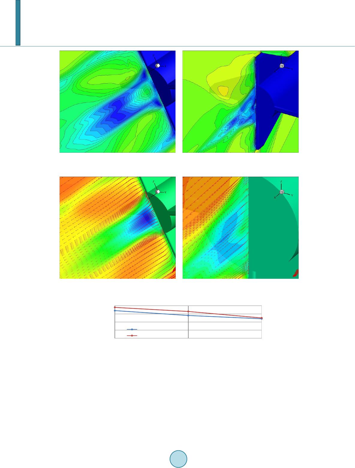
The unsteady compressible flow around a 50 mm projectile governed by the Navier-Stocks (NS)
equation is numerically solved with a Large Eddy Simulation (LES) method, with the Sub-Grid
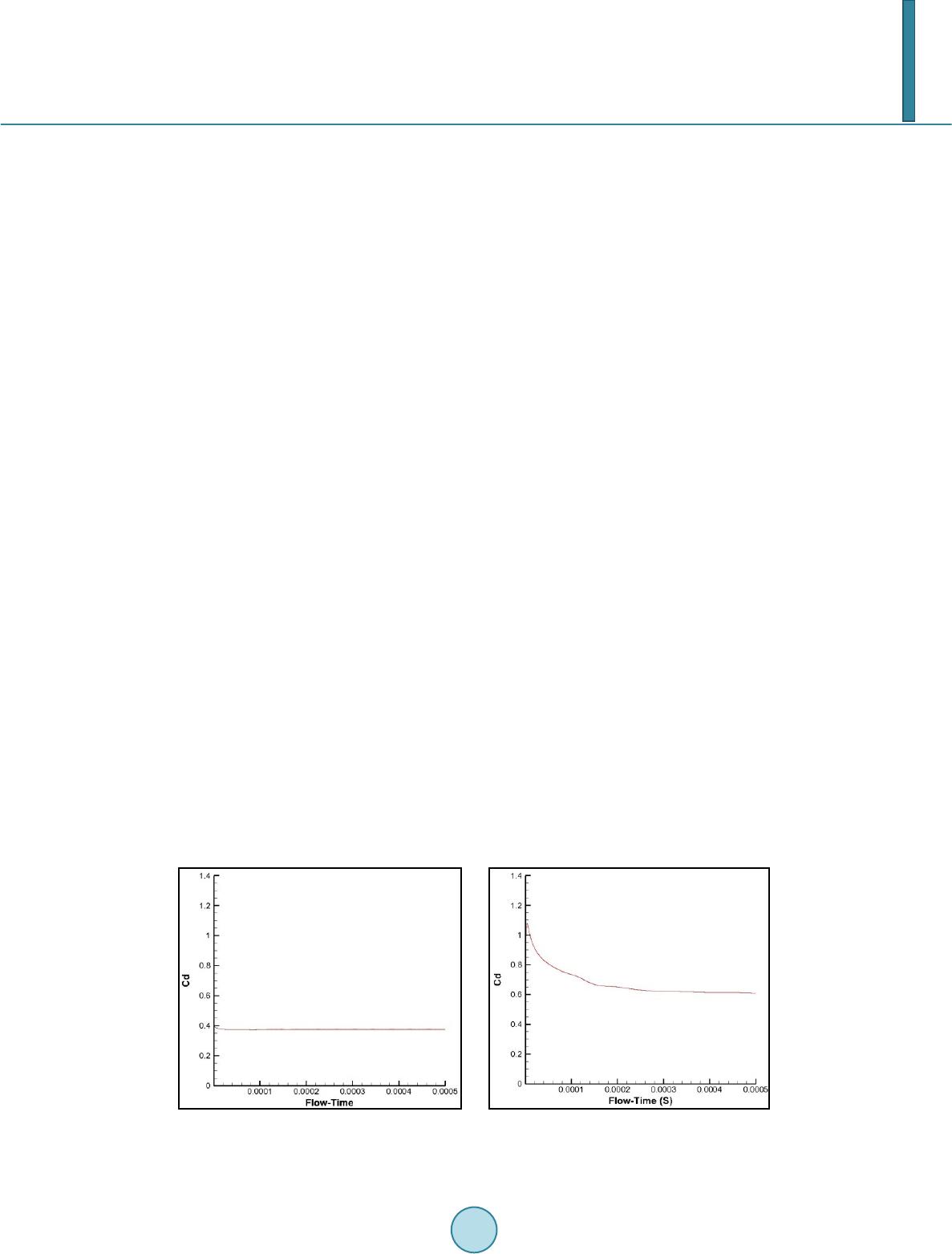
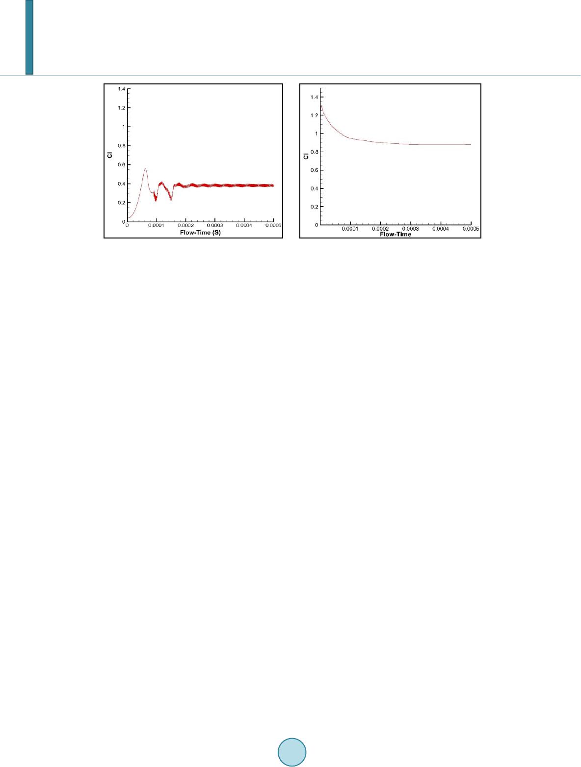
Scale (SGS) solved by Smagorinsky-Lilly model. The computed results are obtained in supersonic
flow regime for a viscous fluid in order to determine the aerodynamic coefficients with different
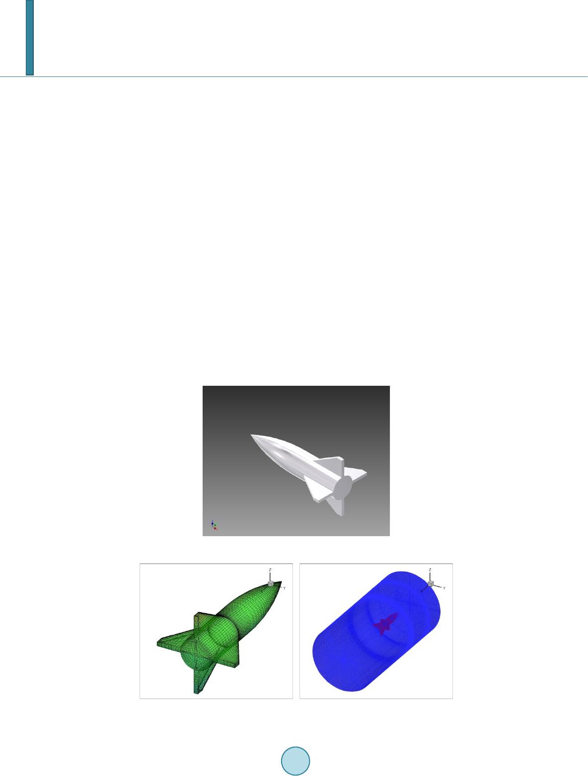
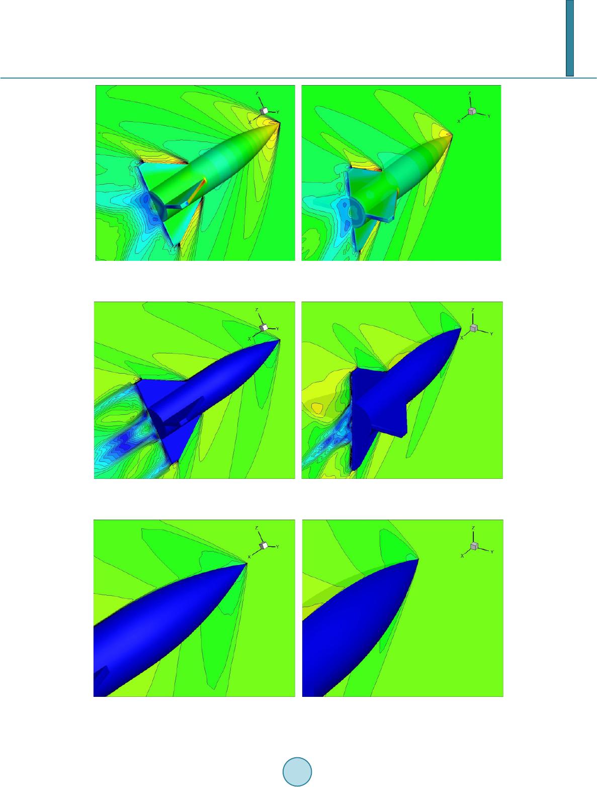
angles of attack. The flow around a body tail projectile was solved as a three-dimensional flow.
Keywords
Body Tail Projectile, Aerodynamic Coefficients, Viscosit y, Flow Field
1. Introduction
The flow around a projectile presents turbulent boundary layers, whose separation is a usual phenomena and a
large turbulent wake formed at the bottom of the object. In ballistic aerodynamics, prevention or control of the
separation of the boundary layer is one of the most important aims, as well as an appropriate ogive design [1] [2].
As it is well known, a turbulent flow carries irregular and fluctuating fluid motions which contribute signifi-
cantly to the transport phenomena. They are always three-dimensional, unsteady and mainly irregular except
perhaps by coherent structures, which are as some kind of organized flow motion that can be recognized in the
instantaneous flow fields as well as in the time-averaged ones [3]. There are also eddies with a wide spectrum of
sizes, from the larger ones close to the flow domain ones, to the much smaller ones at which viscous dissipation
takes place. The numerical techniques available in Computational Fluid Dynamics (CFD) to simulate them can
be split in three main types [4] [5].
i) Direct Numerical Simulation (DNS)
ii) Large Eddy Simulation (LES)
iii) Re ynolds-Averaged Navier-Stokes (RANS)
A LES model is chosen since the Re number range to be considered indicates that the flow is fully turbulent.
Its adoption responds mainly to the computed large-scales, associated to the coherent structures developed due
to the projectile motion. As already stated, the smaller scales are not solved but they are modeled, regarding that
its influence over other scales is related to energy transfers [6]. In this work, the CFD is applied to determine the
aerodynamic coefficients by using a commercial CFD code called FLUENT which solves the governing equa-
*
Corresponding author.
M. E. Wessam et al.
278
tions of the flow motion using a technique of finite volume and takes the meshed computational domain from a
pre-processor program called ICEM-CFD in which the model of the projectile is drawn and the computational
domain is generated and meshed into cells. The implicit segregated structured grid solver was used in these in-
vestigations. Second order upwind discritization was used for the flow variables and turbulent viscosity equa-
tions, furthermore a comparison with experimental data wa s performed. The objective of the present study is to
provide a methodology for the determination of the aerodynamic coefficients of a projectile of given geometry
using the more recent advances in computational fluid dynamic technique. It is convenient to make use of the
more powerful packages and the higher computational capacities that are available today.
2. Computational Fluid Dynamics
2.1. Model Geom etry
The full scale 50 mm projectile with a tapered leading and trailing fin edge and sharp nose tip was modeled in
the CFD simulations Figure 1 [7], in order to determine the aerodynamic coefficients. The projectile was 241
mm long. The nose was tangent ogive. The cylinder body was 111 mm long. The fins were 6.35 mm thick with,
a 38.1 mm span, a 76.2 mm root chord and a 12.7 mm tip chord. The fin trailing edge was flush with the projec-
tile base.
2.2. Grid Generati o n
The grids for the geometry investigated were obtained from ICEM-CFD software as the numerical grids had
been previously constructed each grid was structured and contained mostly hexahedral cells. The projectile con-
tained approximately 1.15 million cells. The computational domain was extended to be 3 times length down-
stream far from projectile base, 2 times length around the projectile, and ¾ times length upstream far from pro-
jectile nose Figure 2.
Figure 1. Projectile geometry.
Figure 2. Meshed projectile and computational domain.
M. E. Wessam et al.
279
2.3. Solve r
The CFD is applied to determine the aerodynamic coefficients by using a commercial CFD code called
FLUENT which solves the governing equations of the flow motion using a technique of finite volume. The
Navier-Stokes equation is numerically solved with a Large Eddy Simulation (LES) method, with the Sub-Grid
Scale (SGS) solved by Smagorinsky-Lilly model. In LES techniques, large eddies are resolved directly, while
small eddies are modeled. Large Eddy Simulation (LES) thus falls between DNS and RANS in terms of the
fraction of the resolved scales. Resolving only the large eddies allows one to use much coarser mesh and larger
times-step sizes in LES than in DNS. However, LES still requires substantially finer meshes than those typically
used for RANS calculations [8]. In addition, LES has to be run for a sufficiently long flow-time to obtain stable
statistics of the flow being modeled; therefore, high-performance computing (e.g., parallel computing) is a ne-
cessity for LES as in the present work. The momentum balance equations are solved with an “effective” kine-
matic viscosity νe= ν + νt, which is the sum of the molecular part calculated as ν = µ/ρ, plus a “turbulent” one νt
[9]. The SGS stresses are approximated by second order Roe scheme.
2.4. Boundary Conditions
The far field boundary (including the inflow and outflow boundaries) is set to pressure far field density-based
inflow/outflow. This boundary condition is a characteristic type that allows the solver to determine the condi-
tions at the far field boundary (inflow, supersonic outflow) and either implicitly sets the boundary condition to
free stream conditions (inflow, supersonic outflow). Free stream pressure and temperature are set to 1 atm and
300 K, respectively. Density is then calculated from the perfect gas assumption. Velocity remained fixed at
Mach number 1.5. Angle of attack is taken as 0° and 10°. For the projectile body and fins, when present, the
boundary condition is set to be a no slip, adiabatic wall.
3. Results and Discussion
Results for case of free stream Mach number M = 1.5 and angle of attack α = 0°, 10° will be analyzed in order to
understand the three-dimensional unsteady compressible flow around a body tail projectile.
3.1. Drag and Lift Convergence History
Figure 3 and Figure 4 show the history of the drag and lift coefficient respectively for the two cases (α = 0° and
α = 10°) with the flow time. For α = 0° drag coefficient had a constant value after about 0.10 ms while the lift
coefficient had a constant value after about 0.15 ms, furthermore the final total drag coefficient obtained is about
0.38 while the final lift coefficient obtained is about 0.38. For α = 10° drag coefficient had a constant value after
about 0.30 ms while the lift coefficient had a constant value after about 0.31 ms, furthermore the final total drag
coefficient obtained is about 0.61 while the final lift coefficient obtained is about 0.88. As the angle of attack
increases, the drag and lift coefficients increase.
(a) (b)
Figure 3. Drag coefficient convergence history for M = 1 .5 . (a) α = 0°; (b) α = 10°.
M. E. Wessam et al.
280
(a) (b)
Figure 4. Lift coefficient convergence history for M = 1.5. (a) α = 0°; (b) α = 10°.
3.2. Contours of Static Pressure Distribution
From Figure 5 it can be noticed that there is no more symmetry distribution of static pressure contours between
upper and lower half of the symmetry plane for α = 10°. The region in which the value of static pressure is lower
than the free stream pressure has a large area at the upper half of the symmetry plane. rather than for α = 0° the
symmetry distribution of static pressure contours between upper and lower half of the symmetry plane is
cleared.
3.3. Contours of Mach Number and Velocity Vector Distribution
Also, from Figure 6 and Figure 7 the Mach number distribution was not symmetric between upper and lower
half of the symmetry plane, the boundary layer build up in the upper half is greater than the lower half that is
because of the presence of the angle of attack. Figur e 8 shows the Mach number distribution behind the base of
the body. The wake region, in which the Mach number is minimum value, is clear from the figure. Figure 9
shows the velocity vector distribution behind the base of the body, in which the vortices are clearly large for α =
10°.
3.4. Comparison between CFD Simulation and Experimental Drag Coefficient
In Exterior Ballistics, the specialty related to projectile flight studies, the drag coefficient curves take a funda-
mental rule for different applications, such as the generation of firing tables. These curves can be obtained also
from tests inside wind tunnels or theoretical calculus. In the first case, the interferences between the projectile or
its model and the tunnel walls affect the precision of results; in the second, the hypothesis adopted could move
the results away from the real behavior. Because of the limitations of the methods mentioned before, a different
way for the making up of these curves is the identification of the aerodynamic properties of an object from flight
test over a real specimen. Figure 10 shows the Comparison between drag coefficient curves obtained by CFD
simulations for 0° angle of attack and Mach number of 1.5, 2, and 3 with the drag curves obtained from [10],
(Axial Force Coefficient vs. Mach number, the baseline data). From Figure 10, the drag coefficient decreased
linearly with Mach number and shows a good agreement with the baseline tested data.
4. Conclusion
3-D unsteady flow CFD simulation around a body tail projectile model were performed at a supersonic Mach
number of 1.5 and angles of attack of 0˚ and 10˚ using a commercial CFD code called (FLUENT 6.3.26) which
solves Navi er-Stokes equation with a Large Eddy Simulation (LES) method. Sub-Grid Scale (SGS) solved by
Smagorinsky-Lilly model, Roe-FDS scheme and a second order discretization were used in this work. A com-
parison were performed for α = 0° and Mach number of 1.5, 2, and 3. These 3-D unsteady CFD investigations
have provided fundamental understanding of flow field around a body.
M. E. Wessam et al.
281
(a) (b)
Figure 5. Contours of static pressure distribution for M = 1.5 {(a) α = 0° and (b) α = 10°}.
(a) (b)
Figure 6. Mach number distribution for M = 1.5 {(a) α = 0° and (b) α = 10°}.
(a) (b)
Figure 7. Mach number distribution nose section for M = 1.5 {(a) α = 0° and (b) α = 10°}.
M. E. Wessam et al.
282
(a) (b)
Figure 8. Mach number distribution base section for M = 1.5 {(a) α = 0° and (b) α = 10°}.
(a) (b)
Figure 9. Velocity distribution base section for M = 1.5 {(a) α = 0° and (b) α = 10°}.
Figure 10. Comparison between CFD simulation and experimental drag coef-
ficient for α = 0° [1 0].
Acknowledgements
This work supported by the Foundation of Key Laboratory of Transient Physics (9140C300205110C30), China.
References
[1] Sahu, J. (1991 ) Transonic Navier-Stokes Computations for a Spinning Body of Revolution. Tech. Rep. ARL-TR-3265,
US Army Research Laboratory.
0
0.1
0.2
0.3
0.4
1.5
2
3
Mach number
experimen t a l
CFD simulation
M. E. Wessam et al.
283
[2] Weinacht, P. (2003) Prediction of Projectile Performance, Stability, and Free-Flight Motion Using Computational Flu-
id Dynamics. Tech. Rep. ARL-TR-3015, Army Research Laboratory.
[3] Townsend, A.A. (1980) The Structure of Turbulent Shear Flow. 2nd Edition, Cambridge Univ. Press.
[4] Rodi, W. (2006) DNS and LES for Some Engineering Flo ws . Fluid Dynamics Research, 38, 145-173.
http://dx.doi.org/10.1016/j.fluiddyn.2004.11.003
[5] Sagaut, P. (2001) Large Eddy Simulation for Incompressible Flows, an Introduction. Springer, Berlin.
[6] Calo, V. (2005 ) Residu al-Based Multiscale Turbulence Modeling: Finite Volume Simulations of Bypass Transition.
Ph.D. Thesi s , Stanford University.
[7] Massey, K.C., McMichael, J., Warnock, T. and Hay, F. (2005) Mechanical Actuators for Guidance of a Supersonic
Projectile. 23rd Applied Aerodynamics Conference, AIAA 2005-4970.
[8] Chapman, D.R. (19 79) Computational Aerodynamics Development and Outlook. AIAA Journal, 17, 1293-1313.
http://dx.doi.org/10.2514/3.61311
[9] Smagorinsky, J. (1963) General Circulation Experiments with the Primitive Equations: I. the Basic Equations. Monthly
Weather Review, 91, 99-164. http:// dx. do i.o rg/ 10. 11 75/ 1520 -0493(1963)091<0099:GCEWTP>2.3.CO;2
[10] Silton, S.I. (2004 ) Mechanical Actuators for Guidance of a Supersonic Projectile. 22nd Applied Aerodynamics Confe-
rence and Exhibit, AIAA 2004-5195.