Journal of Applied Mathematics and Physics, 2014, 2, 269-276
Published Online May 2014 in SciRes. http://www.scirp.org/journal/jamp
http://dx.doi.org/10.4236/jamp.2014.26032
How to cite this paper: Lin, M.-Y., Li, C.-Y. and Wang, A.-P. (2014) Particle Based Simulation for Solitary Waves Passing over
a Submerged Breakwater. Journal of Applied Mathematics and Physics, 2, 269-276.
http://dx.doi.org/10.4236/jamp.2014.26032
Particle Based Simulation for Solitary Waves
Passing over a Submerged Breakwater
Meng-Yu Lin*, Chiung-Yu Li, An-Pei Wang
Department of Civil Engineering, Chung Yuan Christian University, Chung Li 32023
Received Ja nu ary 2014
Abstract
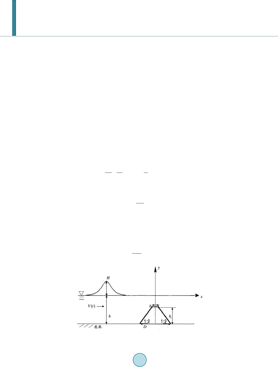
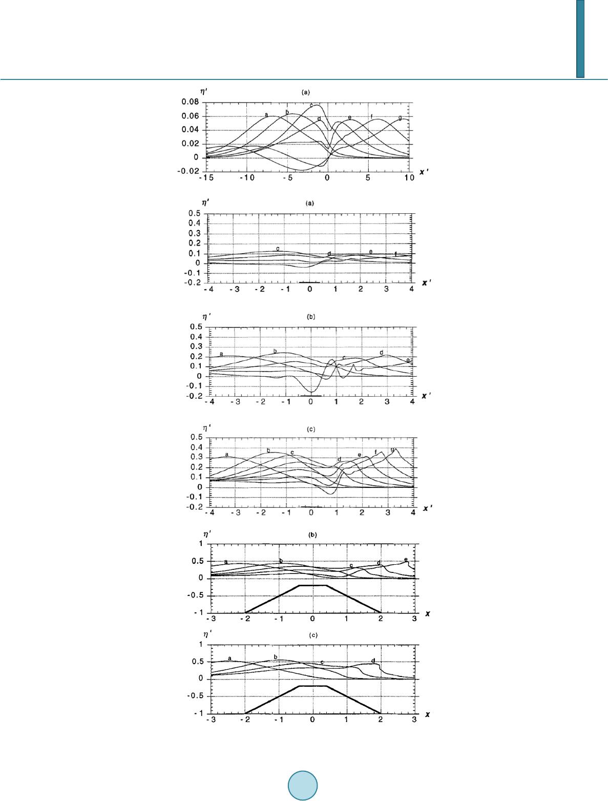
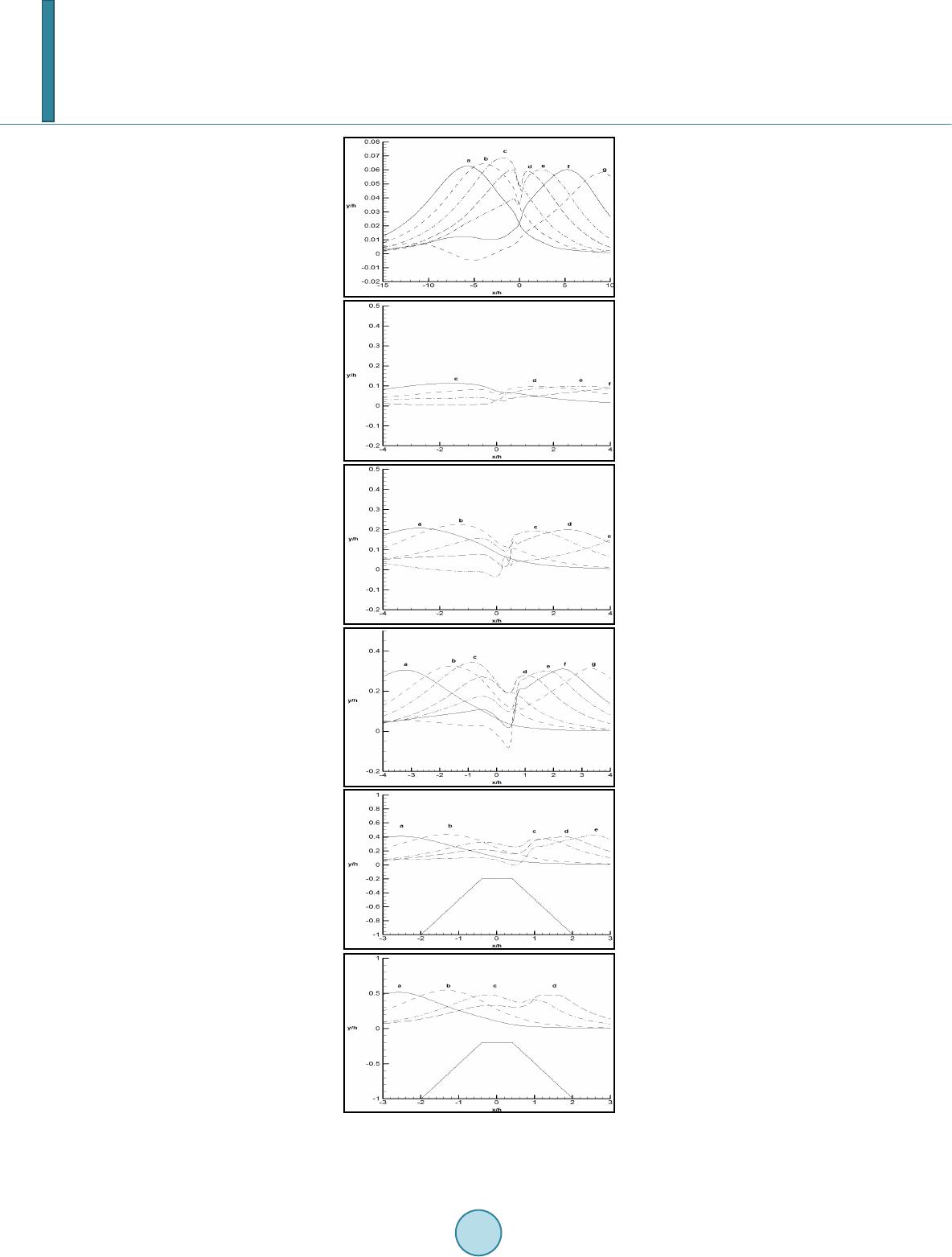
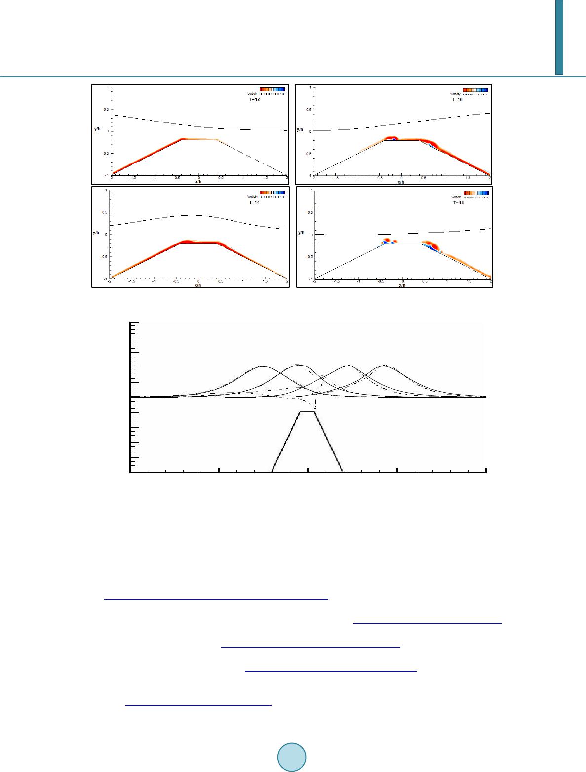
This research develops a two-dimensional numerical model for the simulation of the flow due to a
solitary wave passing over a trapezoidal submerged breakwater on the basis of generalized vortex
method s. In this method, the irrotational flow field due to free surface waves is simulated by em-
ploying a vortex sheet distribution, and the vorticity field generated from the submerged object is
discretized using vortex blobs. This method reduces the difficulty in capturing the nonlinear de-
formation of surface waves, and also concentrates the computational resources in the compact re-
gion with vorticity. This numerical model was validated by conducting a set of simulations for ir-
rotational solitary waves and then compared with the results of a relevant research. The compar-
isons exhibit good agreement. The rotational flows induced by different incident wave height were
simulated and analyzed to study the effect of vorticity on the deformation and the breaking of so-
litary waves.
Keywords
Solitary Wav e , Submerged Breakwater, Vo rtex , Vortex Meth od, Particle Simulation
1. Introduction
The interaction of surface water waves with submerged structures has attracted attention in many fields of engi-
neering applications. Numerous investigations for this problem have been implemented based on potential-flow
theory with the assumption that the flow is irrotational. For example, [1] employed a boundary element method
to establish a two-dimensional numerical model for the simulation of surface waves in an irrotational, inviscid
fluid flow, and then simulated the breaking of solitary waves passing over a trapezoidal submerged breakwater.
One of the benefits of the approaches using the irrotational-flow assumption is the efficient computation by ap-
plying boundary integral methods, and these approaches usually predict the transformation of water waves ac-
curately if flow separation is not severe. For many engineering problems the effects of flow separation should
not be ignored; therefore, the studies using potential-flow theory usually only investigate the scattering of sur-
face waves (see, e.g., [2]-[4]).
This research develops a two-dimensional numerical model for the simulation of the flow due to a solitary
*Corresponding author.

M.-Y. Lin et al.
270
wave passing over a trapezoidal submerged breakwater on the basis of generalized vortex methods. The main
object of this research is to gain insight into the deformation of free surface as well as the shedding of vortices
from the breakwater. In this study an essentially grid-free numerical model is developed. The motivation is
based on the fact that in water-wave problems the flow field far from submerged bodies can be simplified to be
irrotational and may be treated by including a viscous-flow correction to the potential-flow analysis. To accom-
plish this, we apply the Helmholtz decomposition to decompose the flow field into two components: one related
to the vorticity (vortical velocity) and the other being irrotational. The potential flow with surface waves is
solved by employing a generalized vortex sheet approach, and the viscous flow is solved via a Lagrangian vor-
tex particle method. In contrast with grid-based schemes, the Lagrangian vortex particles convect without nu-
merical dissipation and automatically adjust to resolve the regions with vorticity.
2. Mathematical Formulations
2.1. Governing Equations
The problem of interest concerns the calculation of the two-dimensional flow of a solitary wave over a near-wall
circular cylinder in a uniform channel. The viscous effects as well as the generation of vorticity at the free sur-
face are ignored. The x-axis lies in the undisturbed free surface and the y-axis points vertically upward with unit
vectors
ˆx e
an d
ˆ
y
e
, respectively (see Figure 1). The corresponding fluid velocity components are u and v re-
spectively, and
u
is the fluid velocity vector. The motion of the fluid is governed by the incompressible Navi-
er-Stokes equations:
0∇⋅= u
(1)
2
D1
ˆ
·
Dp tg t
υ
ρ
==− ∇−
∂∇ ++
∂∇
uu juu u
(2)
where p is the fluid pressure,
ρ
is the density of fluid, g is the gravitational acceleration, and
ν
is the kine-
matic viscosity. In velocity-vorticity form, above equations can be expressed by the vorticity transport equation:
2
D
Dt
ωυω
= ∇
(3)
whe re
ˆ·
ω = ∇×ju
is the vorticity field with the unit vector
ˆ
j
out of the page.
2.2. Boundary Conditions
At the free surface, the flow field satisfies the kinematic and dynamic boundary conditions, which can be ex-
pressed in a Lagrangian description as
D()
D
f
f
t=xu
x
(4)
Figure 1. Definition sketch of the problem.

M.-Y. Lin et al.
271
D1
ˆ
()
D
fa
pg
t ρ
=−∇−x
uj
(5)
On solid boundaries (at the seabed or the boundary of the cylinder)
b
S
, no-slip boundary condition is em-
ployed:
on S
b
0 u=
(6)
3. Generalized Vortex Meth o ds
If the interface between air and water is not perpendicular to the pressure gradient, vorticity will be generated
and must be confined to the interface at all times because of the absence of free-surface viscosity. The so-called
generalized vortex sheet approach for interfacial waves is the basis for several different computational methods
[5]-[7].
The flow field studied in this research is generated by the free-surface waves and the vorticity separated from
the circular cylinder and the seabed. By applying the integral formulations of the Helmholtz decomposition [8],
the integral representation for the velocity field has the form:
()()()()() ,
f
VS
dd ωγ
′′′′ ′′
=− +−
∫∫
uxKx xxxKxxxx
(7)
where V is the volume of fluid, Sf denotes the free surface, γ is the strength of a vortex sheet at the free surface,
and
2
( ,)
() 2||
yx
π
−
=Kx x
(8)
In (7), The first integral represents the rotational flow field induced by vorticity, and the second integral
represents the irrotational flow field induced by the vortex sheet along the free surface. The vortex sheet strength
γ is related to the tangential velocity jump across the free surface:
12
() γ =−⋅
uus

(9)
where u1 and u2 are the limiting values of the velocity vector below and above the free surface, respectively, and
ˆ
s
is a unit vector oriented tangent to the vortex sheet (see Figure 2).
From the integral representation shown in (7) with the vorticity transport Equation (3) and the evolution equa-
tion for γ derived from the dynamic free surface boundary condition (5), an alternative problem can be con-
structed for solving xf, ω and γ rather than the original problem with primitive variables xf, u and p. The flow
field evolves by following the trajectories of the vorticity-carrying elements xω and the free-surface points xf,
and then updating their strengths based on the following sets of equations. For vorticity ω,
d
dt
ω
=
xu
(10)
2
d
dt
ωνω
= ∇
(11)
and for vortex sheet γ,
Figure 2. Vortex sheet along the free surface.

M.-Y. Lin et al.
272
f
f
d
dt =
xu
(12)
22
f
f
dg
dt s
γγ
∂
=− ⋅++
∂⋅⋅
usa sjs
 
(13)
where af is the averaged velocity across the free surface, and
2
1( )
8
f
f
d
dt s
γ ∂
= +⋅⋅ ∂
u
as s

(14)
The vorticity field ω is determined by applying a Lagrangian vortex particle method to obtain a numerical ap-
proximation in terms of N vorticity-carrying particles
1
( ,)(())()
N
jj
j
t tt ωη
=
= −Γ
∑
x xx

(15)
Each particle is identified by its position, xj and its circulation, Γj. The regularized function ηε is the Gaussian
distribution:
2
22
1
( )exp
22
ηπ

 = −


x
x


(16)
The velocity of the particle at xj is
1
( )()()()
f
N
jj iij
S
i
d γ
=
=− Γ+−
∑∫
ux KxxKxxxx

(17)
whe re
2
2
||
()()1 exp2


= −−





x
K xKx


(18)
4. Model Validation
To validate the present model, we simulate the flow problem that was investigated in [1] using a boundary ele-
ment method, and then compare the results of two computations. The simulated region is shown in Figure 1,
where H is the wave height, h the still-water depth, D and b the width of the bottom and the top of the breakwa-
ter, respectively, and h1 the height of the breakwater. In all computations
0.2bh=
,
0.4Dh=
and
10.8hh=
.
The cases of relative wave height H/h = 0.06, 0.1, 0.2, 0.3, 0.4 and 0.5 are simulated. Since the simulations in [1]
ignore viscous effects, in the computations using the proposed model presented in this section the effects of vis-
cosity and the generation of vorticity are also ignored.
Figure 3 shows the computational results in [1] for the evolution of the free surface passing over the break-
water under different wave height, and Figure 4 is the corresponding results computed by the present model.
The evolution of the solitary wave in each case predicted by the present model is seen to be in fairly agreement
with the results in [1]. The small discrepancy between two simulations is because that two models employ dif-
ferent method to generate the solitary wave.
5. Results and Discussion
Figure 5 shows the vorticity fields at indicated times for H/h = 0.4. When the wave crest is on the top of the
breakwater (t = 14), the shear layers at the left and the right side of the breakwater separate from the wall and
then generate vortices into the flow. When the wave crest is leaving (t = 16), the vortices at the left and right
corner of the breakwater form recirculating regions and then induce secondary vortices on the wall. When the
wave crest moves away from the breakwater (t = 18), the vortices dissipate gradually due to viscous effect be-
cause the driven flow disappears.
To investigate the effect of vorticity on the transformation of free surface, the comparison between the com-
puted free surface transformation with and without vorticity effect is shown in Figure 6. Since the vortices

M.-Y. Lin et al.
273
Figure 3. Computed results for solitary wave transformation in [1].

M.-Y. Lin et al.
274
Figure 4. Solitary wave transfor matio n com-
puted by the present model.

M.-Y. Lin et al.
275
Figure 5. Vorticity fields at indicated times for H/h = 0.4.
Figure 6. Comparison of free surface transformation for H/h = 0.4 (−: rotational flow; - -: irrotational flow).
form recirculating regions on the wall of the breakwater, the severe deformation of free surface in the case of ir-
rotational computation do not occur in the case with vorticity effect.
References
[1] Grilli, S.T., Losada, M.A. and Martin, F. (1994) Characteristics of Solitary Wave Breaking Induced by Brea kwaters.
Journal of Waterway Port Coastal and Ocean Engineering-ASCE, 120, 609-628.
http://dx.doi.org/10.1061/(ASCE)0733-950X(1994)120:6(609)
[2] Yenug, R.W. and Vaidhyanathan, M. (19 92 ) N on-Linear Interaction of Water Waves with Submerged Obstacles. In-
ternational Journal for Numerical Methods in Fluids, 14, 1111-11 30 . http://dx.doi.org/10.1002/fld.1650140907
[3] Gobbi, M.F. and Kirby, J.T. (199 9 ) Wave Evolution over Submerged Sills: Tests of H igh -Order Boussinesq Model.
Coastal Engineering, 37, 57-96. http://dx.doi.org/10.1016/S0378-3839(99 )00 015 -0
[4] Guyenne, P. and Nicholls, D.P. (2005) Numerical Simulation of Solitary Waves on Plane Slopes. Mathematics and
Computers in Simulation, 69, 269-281. http://dx.doi.org/10.1016/j.matcom.2005.01.005
[5] Longuet-Higgin s, M.S and Cokelet, E.D (1976) The Deformation of Steep Surface Waves on Water. I. A Numerical
Method of Computation. Proceedings of the Royal Society of London. A. Mathematical and Physical Sciences, 350,
1-26. http://dx.doi.org/10.1098/rspa.197 6. 0092
-10 -50510
-1
-0.8
-0.6
-0.4
-0.2
0
0.2
0.4
0.6
0.8
1
y/h
x/h
T= 12 14 1618

M.-Y. Lin et al.
276
[6] Baker, G.R., Meir on , D.I. and Orszag, S.A. (1982) Generalized Vortex Methods for Free-Surface Flow Problems.
Journal of Fluid Mechanics, 123, 477-501. http://dx.doi.org/10.1017/S0022112082003164
[7] Tr yggva so n, G. (198 8) Numerical Simulations of the Rayleigh-Taylor Instability. Journal of Computational Physics,
75, 253-282. http://dx.doi.org/10.1016/0021-9991(88)90112-X
[8] Li n , M.-Y. and Huang, L.-H. (2009) Study of Water Waves with Submerged Obstacles Using a Vortex Method with
Helmholtz Decomposition. International Journal for Numerical Methods in Fluids, 60, 119-148.
http://dx.doi.org/10.1002/fld.1873