Atmospheric and Climate Sciences, 2011, 1, 33-47
doi:10.4236/acs.2011.12004 Published Online April 2011 (http://www.SciRP.org/journal/acs)
Abrupt Climate Regime Shifts, Their Potential
Forcing and Fisheries Impacts
Alfred M. Powell Jr.1, Jianjun Xu2*
1NOAA/NESDIS/Center for Satellite Applications and Research (STAR), Camp Springs, Maryland
2IMSG at NOAA/ N ESDIS/Star, Camp Sprin gs , Maryland
Received February 9, 2011; revised March 14, 2011; accepted March 21, 2011
Abstract
The purpose of this paper is to investigate whether a logical chain of events can be established to explain the
abrupt climatic regime shift changes in the Pacific that link the atmosphere to the ocean to fisheries impacts.
The investigation endeavors to identify synchronous abrupt changes in a series of data sets to establish the
feasibility of abrupt of climate change often referred to as regime shifts. The study begins by using biological
(fish catch/stock) markers to mathematically identify the dates of abrupt change. The dates are confirmed by
a literature search of parameters that also show abrupt changes on the same dates. Using the biological date
markers of abrupt change, analyses are performed to demonstrate that the interactions between the atmos-
phere, ocean, ecosystems and fisheries are a plausible approach to explaining abrupt climate change and its
impacts.
Keywords: Climate Regime Shift, Fishery
1. Introduction
A number of fish stock studies have identified the ap-
parent synchronous nature of many of the world’s largest
fish stocks (Food and Agriculture Organization (FAO),
United Nations Fisheries Circular No. 920). These stud-
ies include the rise and fall of sardines in widely sepa-
rated areas of the Pacific [1], as well as the out-of-phase
nature of sardines and anchovies in multiple locations
globally [2-5]. Based on the sardine/anchovy analysis,
Chavez et al. [2] pointed out the abrupt changes in fish
populations are difficult to explain on the basis of fishing
pressure. Lehodey et al. [6] stated that fish population
variability is clos ely related to environmental variability.
In addition, he also points out that the low frequency
population variability was first observed in small pe lagic
fish like sardines and anchovies but similar variability
has been shown in larger fish like salmon, groundfish
and tuna which track well with large scale climate pat-
terns like the Pacific Decadal Oscillation (PDO) and the
North Atlantic Oscillation (NAO). Chavez et al. [2] fur-
ther remarked that the mechanism(s) responsible for the
abrupt regime shifts should be relatively direct and sim-
ple, similar in the different regions, and likely linked
with large-scale atmospheric and oceanic forcing.
The purpose of this research is to search for the
large-scale forcing by identifying specific changes in the
atmosphere, ocean and ecosystems that could offer a
physical explanation for the chain of environmental in-
teractions that could cascade through the system and
affect the fisheries. The data and methodology are de-
scribed in the next section and is followed by how the
regime shifts were identified. Prior to the detailed analy-
sis synopsis, background information on the global at-
mospheric wave pattern is provided for the multidisci-
plinary audience of readers. The analysis uses both a
mathematical appro ach combined with a literature search
to define the likely years of regime shifts. Based on the
regime shift period identification, a top-down analysis
(from atmosphere to ocean to fish) is performed to dem-
onstrate regime shifts in the atmosphere can lead to wind
stress changes. The wind stress impacts on ocean tem-
peratures are shown with the consequential changes in
fisheries impacts identified.
2. Data and Methodology
2.1 Data
The data used in this study include California’s fishery

A. M. POWELL ET AL.
34
landing data published by the California Department of
Fish and Game (CDFG), reanalysis data sets created by
the National Centers for Environmental Prediction
(NCEP), the National Center for Atmospheric Research
(NCAR) and sea surface temperature data produced by
the National Climatic Data Center (NCDC) of the Na-
tional Oceanic and Atmospheric Administration (NOAA).
1) California’s fish landing data
The landings of California’s fishery catch brought to
shore are record ed b y fish buyers , markets, an d canneries
and compiled by CDFG [7]. The annual commercial
landings of fish and invertebrates are taken from the
Southwest Fisheries Science Center located in the Pacific
Fisheries Environmental Laboratory of NOAA. To track
the variability of species from California’s borders, this
data set includes only the landing s recorded as caug ht off
California. The data sp ans the years 1928 to 2008. While
the initial year for the raw data set was 1928, the initial
record for each species starts from different times. The
data includes the total catch for 31 marine species. The
thirty one species are listed in Table 1.
2) NCEP-NCAR reanalysis
The monthly NCEP-NCAR reanalysis [8] with a 2.5˚
× 2.5˚ grid resolution is used for the periods of 1948-
2008. It should be noted that the reanalysis period of
1948-1978 has no satellite data. The Television Infrared
Observation Satellite (TIROS) Operational Vertical
Sounder (TOVS) data, the Microwave Sounding Unit
(MSU), the High Resolution Infrared Radiation Sounder
(HIRS) and the Stratospheric Sounding Unit (SSU) in-
formation were no t available be fore the end of 197 8. The
Special Sensor Microwave/Imager (SSM/I) data was
assimilated in this system from 1993. The geopotential
height and wind fields are used in the study.
Table 1. List of the 32 category names for California fish
landings 1.
Name Code number Name Code number
all 1 sanddab 17
barracuda 2 sardine 18
bass-giant 3 scorpionfish 19
bonito 4 shark 20
cabezon 5 sheephead 21
croaker-white 6 skate 22
flounder 7 smelt 23
halibut 8 sole 24
herring 9 swordfish 25
lingcod 10 tuna-albacore 26
mackerel-Jack 11 tuna-bluefin 27
mackerel-chub 12 tuna-skipjack 28
perch 13 turbot 29
rockfish 14 whitefish 30
sablefish 15 whiting 31
salmon 16 yellowtail 32
3) NCDC Extended Reconstructed Sea Surface Tem-
peratures
The latest version of the Extended Reconstructed Sea
Surface Temperatures (ERSST.v3) is used in this study,
which is generated using in-situ SST data and improved
statistical methods that allow stable reconstruction using
sparse data. The monthly analysis extends from January
1854 to the present, but because of sparse data in the
early years, the analyzed signal is damped before 1880.
After 1880, the strength of the signal is more consistent
over time. ERSST is suitable for long-term global and
basin wide studies; local and short-term variations have
been smoothed in ERSST.
4) International Comprehensive Ocean-Atmosphere
Data Set (ICOADS)
The International Comprehensive Ocean-Atmosphere
Data Set (ICOADS) offers surface marine data spanning
the past three centuries, and simple gridded monthly
summary products for 2˚ latitude  2˚ longitude boxes
back to 1800 (and 1˚ × 1˚ boxes since 1960). As it con-
tains observations from many different observing sys-
tems encompassing the evolution of measurement tech-
nology over hundreds of years, ICOADS is probably the
most complete and heterogeneous collection of surface
marine data in existence.
2.2. Methodology
The geopotential height fields from the NCEP-NCAR
reanalysis were decomposed into Fourier harmonics and
the Fourier coefficients were used to recompose the
temporal field for single zonal waves. Wavenumbers 1-6
are Fourier deco mposed fro m the 61-yr (1948-2008 ) data.
The wave height pattern anomaly is created by subtract-
ing the mean heights for each wave from the original
height average. Finally, using the fish landing analysis,
the northern hemispheric wave pattern was analyzed to
determine whether the typical cause-effect mechanism
(atmospheric forcing, ocean change and fishery changes)
could explain any potential linkages between the data
sets and the regime shift dates.
3. Northern Hemispheric Wave Pattern
Background
Meteorologists monitor the wave pattern by tracking the
high and low pressure systems which are associated with
fair and inclement weather respectively. The northern
hemispheric wave pattern is used by forecasters to help
predict future changes several days ahead. On a constant
pressure surface, contouring the height of the pressure
surface indicates the regions of counterclockwise winds
(low pressure systems) and clockwise winds (high pres-
sure systems). The winds blow parallel to the height
contours above the boundary layer. Figure 1 shows two

A. M. POWELL ET AL.
35
(a)
(b)
Figure 1. Pattern of geopotential height (gpm) at 500 hPa in
(a) January 01, 2007 and (b) January 20, 2007.
different states of the wave pattern in the middle of the
troposphere on different days. The point of this graphic
is to demonstrate that when the pattern changes, its im-
pacts will be felt around the world. The dashed lines on
the figure represent ‘troughs’ (low pressure systems) or
regions where significant weather can be expected.
While these patterns shift daily, there is an overall mean
state.
An analysis of the last 50 years of data contained in
the NCEP-NCAR reanalysis was accomplished by Pow-
ell and Xu [9]. The analysis was performed in an attempt
to discriminate between potential climatological or de-
cadal wave states. In their analysis, the ten strongest
(top-10) amplitu de waves and the ten weakest (weak-10 )
amplitude waves over the 50-year period were analyzed
for common characteristics. Figure 2 is based on their
(a)
(b)
(c)
Figure 2. Stratospheric height climatology, and the com-
posite stratospheric height (30 hPa) during the top 10
strongest and weakest amplitude planetary wave years in-
corporating wavenumbers 1 thru 5. (a) climatology, (b)
anomaly in top 10 strongest years, (c) anomaly in top 10
weakest years.

A. M. POWELL ET AL.
36
work and shows wavenumbers 1-5 for the strong-10
wave pattern with its positive anomaly (difference from
the mean state) over the polar Pacific and its negative
anomaly over the polar Atlantic similar to the clima-
tological wave pattern. For the weak-10 waves, see Fig-
ure 2 where the stratospheri c hei g ht climatology , and the
composite stratospheric height ( 30 hPa) du ring th e top 10
strongest and weakest amplitude planetary wave years
incorporating wavenumbers 1 thru 5 are shown (a) cli-
matology, (b) anomaly in top 10 strongest years, (c)
anomaly in top 10 weakest years anomaly. This pattern
was essentially a reversal of the climatological anomaly
(a change of phase) occurs between the strongest and
weakest wave energies. This indicates that changes in the
northern hemispheric wave pattern may affect every
ocean and land mass at approximately the same time in a
manner that can be readily analyzed.
More specifically, Figure 2 shows the climatological
mean state for the period 1948-2008 for wavenumbers
1-5 at 30 hPa. The longest atmospheric wave (wave
-number 1) can be represented by one low (trough) and
one high (ridge) pressure area as it circles the globe.
Wavenumber 1 is also the atmospheric wave with the
most energy and greatest amplitude. As a result, the
northern hemispheric wave pattern anomalies predomi-
nantly reflect changes in wavenumber 1 and this infor-
mation will be used to interpret changes in the regime
shift periods.
In this research, the focus is to determine how the ‘av-
erage state’ between regime shifts may have been af-
fected over decadal length periods. Decadal changes in
the atmospheric waves will affect the winds and tem-
peratures around the globe and provide time for a sig-
nificant response to develop. Each region could be af-
fected differently depending on the wind speed, the wind
direction relative to the coastline, and other factors like
atmospheric stability for example. In this instance, the
physical atmospheric changes (wave amplitude, wave
phase, and its impact on surface wind stress) and the re-
sponse of the ocean to the changing surface stress is
analyzed in a simple and direct fashion. This simple
linkage is thought to be the most likely way the wave
pattern will affect the ocean system and subsequ ently the
ocean ecosystems.
Changes in the northern hemispheric wave pattern
have been associated with the Pacific Decadal Oscilla-
tion (PDO) and the North Pacific Index (NPI). The Pa-
cific Decadal Oscillation is defined as the leading prin-
cipal component (PC) of the monthly SST anomalies in
the North Pacific Ocean [10] and the North Pacific Index
is defined as the area-weighted sea level pressure over
the region 30 ° N - 6 5° N , 16 0° E - 14 0° W [11 ]. Bo th th e
PDO and the NPI reflect changes in the northern hemi-
spheric wave pattern and their potential influence on the
Pacific ocean. The PDO and NPI have been used by nu-
merous authors [12,13 and references therein] as an in-
dication of possible connections or forcings related to
various physical and biological parameters. Since the
PDO and NPI are related to the northern hemispheric
wave pattern, it makes sense that many correlations (both
and positive and negative) have been associated with
these indices. For this analysis, more detail than can be
provided by an index is required. As a result, this re-
search has centered on the actual wave pattern and its
decomposition via Fourier components - in particular
wavenumbers 1-6. By comparing wave pattern changes
attributed to the strongest atmospheric waves, it may be
possible to discern significant wave pattern changes, and
the winds associated with them. As the winds change, the
coupling to the ocean will be affected along with the
ocean ecosystems. This simple, direct, and brief sum-
mary provides the foundation for the following abrupt
climate regime shift analysis.
4. Identification of the Regime Shifts
Numerous studies [12,13 and references therein] have
used the PDO and NPI in their analyses in an attempt to
demonstrate when a regime a shift will occur. Periods
where the PDO and NPI indices cross over the ‘zero’
point tend to be favorite location s in the graphs for iden-
tifying possible regime shifts. The question is whether or
not changes in these indices adequately reflect the im-
pacts on regional ecosystems. Figure 3 shows both the
PDO and NPI indices graphed together in (b). The corre-
lation coefficient between the PDO and NPI is approxi-
mately 0.72 and indicates it accounts for approximately
51% of the variability between the two indices. This im-
plies both indices are likely measuring essentially the
same core atmospheric variation. However, when the two
indices are compared against the fish landing data from
NOAA’s Southwest Fisheries Science Center, the corre-
lation of the fish catch with the PDO is only 0.11 (ac-
counting for only 1 .2% of the varian ce in th e fish land ing
data) and is only 0.03 for the NPI (accounting for
0.0009% of the variance in the fish landing data). One
would expect a much greater correspondence between
the PDO and NPI with the fish landing data if they had a
significant cause-effect relationship. Another possibility
is that the fish catch and wave amplitudes are directly
related and the correlation analysis with the PDO and
NPI indices does not reflect the relationship adequately.
One outcome of this analysis will be to ascertain wh ether
the PDO/NPI indicies are robust enough to reflect the
association between the oceans and fisheries for a spe-
cific basin like the Pacific, or whether a more detailed
analysis is required to assess linkages between the at
mosphere, ocean and fisheries.

A. M. POWELL ET AL.
37
To determine whether a stronger cause-effect rela-
tionship can be ascertained, a series of simple and direct
observational analyses will be performed. The first step
in the analysis process is developing a consistent ap-
proach for id entifying the abrupt climate shifts. Once the
shifts were identified then an analysis was performed by
aggregating the data between the identified regime shift
dates to understand the regime differences. By analyzing
the approximately decadal length changes, an interpreta-
tion about the forcing mechanism(s) can be made.
To identify the regime shifts, the fish landing data
were analyzed for abrupt shifts using the period means
similar to Lehodey [6]. Figure 4 shows the results of the
analysis with regime shifts occurring at approximately
(a)
(b)
Figure 3. Time series of (a) normalized amounts of the total fish landing of California ports and (b) Pacific Decadal Oscilla-
tion (PDO) and North Pacific index (NPI). The correlations are calculated between these time series. The dashed line indicats
the time of regime shift occurrence.
Figure 4. Normalized California’s fish landings from 1928-2008 for total amounts of the 31 fish species. The heavy line indi-
cates the decadal average for the periods of 1928-1947, 1948-1964, 1965-1977, 1978-1988 , 1989-1998 and 1999-2008.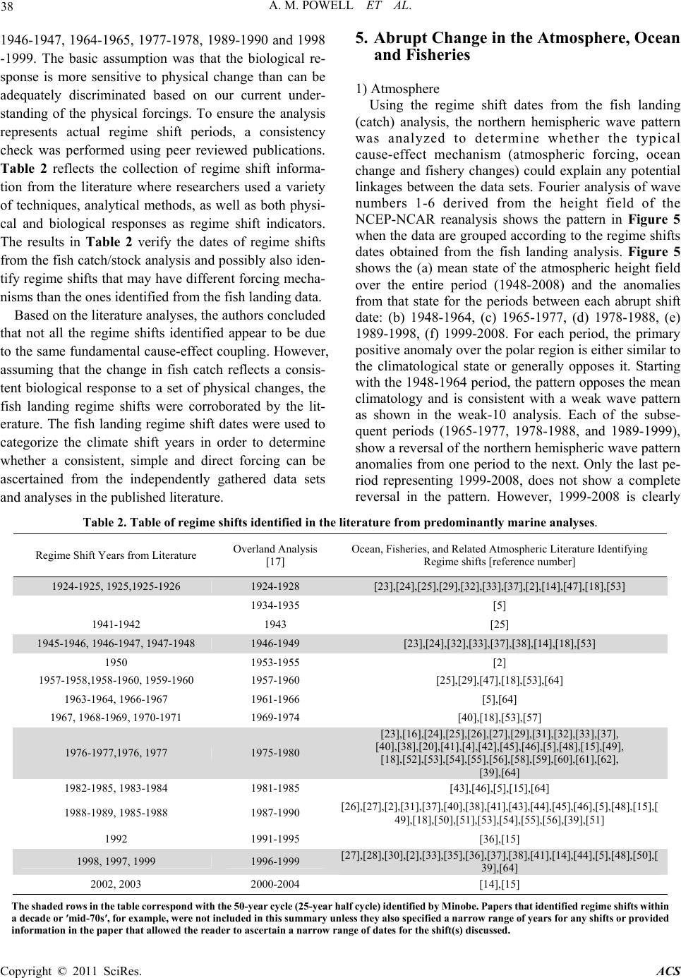

A. M. POWELL ET AL.
38
1946-1947, 1964-1965, 1977-1978, 1989-1990 and 1998
-1999. The basic assumption was that the biological re-
sponse is more sensitive to physical change than can be
adequately discriminated based on our current under-
standing of the physical forcings. To ensure the analysis
represents actual regime shift periods, a consistency
check was performed using peer reviewed publications.
Table 2 reflects the collection of regime shift informa-
tion from the literature where researchers used a variety
of techniques, analytical methods, as well as both physi-
cal and biological responses as regime shift indicators.
The results in Table 2 verify the dates of regime shifts
from the fish catch/stock analysis and possibly also iden-
tify regime shifts that may have different forcing mecha-
nisms than the ones identified from the fish landing data.
Based on the literature analyses, the au thors conc luded
that not all the regime shifts identified appear to be due
to the same fundamental cause-effect coupling. However,
assuming that the change in fish catch reflects a consis-
tent biological response to a set of physical changes, the
fish landing regime shifts were corroborated by the lit-
erature. The fish landing regime shift dates were used to
categorize the climate shift years in order to determine
whether a consistent, simple and direct forcing can be
ascertained from the independently gathered data sets
and analyses in the published literature.
5. Abrupt Change in the Atmosphere, Ocean
and Fisheries
1) Atmosphere
Using the regime shift dates from the fish landing
(catch) analysis, the northern hemispheric wave pattern
was analyzed to determine whether the typical
cause-effect mechanism (atmospheric forcing, ocean
change and fishery changes) could explain any potential
linkages between the data sets. Fourier analysis of wave
numbers 1-6 derived from the height field of the
NCEP-NCAR reanalysis shows the pattern in Figure 5
when the data are grouped according to the regime shifts
dates obtained from the fish landing analysis. Figure 5
shows the (a) mean state of the atmospheric height field
over the entire period (1948-2008) and the anomalies
from that state for the periods between each abrupt shift
date: (b) 1948-1964, (c) 1965-1977, (d) 1978-1988, (e)
1989-1998, (f) 1999-2008. For each period, the primary
positive anomaly over the polar region is either similar to
the climatological state or generally opposes it. Starting
with the 1948-1964 period, the pattern opposes the mean
climatology and is consistent with a weak wave pattern
as shown in the weak-10 analysis. Each of the subse-
quent periods (1965-1977, 1978-1988, and 1989-1999),
show a reversal of the northern hemispheric wave pattern
anomalies from one period to the next. Only the last pe-
riod representing 1999-2008, does not show a complete
reversal in the pattern. However, 1999-2008 is clearly
Table 2. Table of regime shifts identified in the literature from predominantly marine analyses.
Regime Shift Years from Literature Overland Analysis
[17] Ocean, Fisheries, and Related Atmospheric Literature Identifying Regime shifts [reference number]
1924-1925, 1925,1925-19 26 1924-1928 [23],[24],[25],[29],[32],[33],[37],[2],[14],[47],[18],[53]
1934-1935 [5]
1941-1942 1943 [25]
1945-1946, 1946-1947, 1947-1948 1946-1949 [23],[24],[32],[33],[37],[38],[14],[18],[53]
1950 1953-1955 [2]
1957-1958,1958-1960, 1959-1960 1957-1960 [25],[29],[47],[18],[53],[64]
1963-1964, 1966-1967 1961-1966 [5],[64]
1967, 1968-1969, 1970-1971 1969-1974 [40],[18],[53],[57]
1976-1977,1976, 1977 1975-1980
[23],[16],[24],[25],[26],[27],[29],[31],[32],[33],[37],
[40],[38],[20],[41],[4],[42],[45],[46],[5],[48],[15],[49],
[18],[52],[53],[54],[55],[56],[58],[59],[60],[61],[62],
[39],[64]
1982-1985, 1983-1984 1981-1985 [43],[46],[5],[15],[64]
1988-1989, 1985-1988 1987-1990 [26],[27],[2],[31],[37],[40],[38],[41],[43],[44],[45],[46],[5],[48],[15],[
49],[18],[50],[51],[53],[54],[55],[56],[39],[51]
1992 1991-1995 [36],[15]
1998, 1997, 1999 1996-1999 [27],[28],[30],[2],[33],[35],[36],[37],[38],[41],[14],[44],[5],[48],[50],[
39],[64]
2002, 2003 2000-2004 [14],[15]
The shaded rows in the table correspond with the 50-year cycle (25-year half cycle) identified by Minobe. Papers that identified regime shifts within
a decade or ′mid-70s′, for example, were not included in this summary unless they also specified a narrow range of years for any shifts or provided
information in the paper that allowed the reader to ascertain a narrow range of dates for the shift(s) discussed.

A. M. POWELL ET AL.
39
(a) (b) (c)
(d) (e) (f)
Figure 5. Reconstructed planetary wave pattern using geopotential height and wavenumbers 1-6 at 50hPa in NCEP/NAR
reanalysis. (a) Mean of 1948-2008, and the anomalies for each of the following periods: (b) 1948-1964, (c) 1965-1977, (d)
1978-1988, (e) 1989-1998; (f) 1999-2008. Units: gpm. Shaded areas indicate positive anomalies.
weaker in terms of the magnitud e of the anomalies. Also,
the 1999-2008 period may be too long since another re-
gime shift was possibly iden tified in 2003 [14,15]. Since
the wind patterns will change in accordance with these
shifts in atmospheric wave pattern anomalies, it is rea-
sonable to assume the ocean will show corresponding
signs of change. The northern hemispheric wave pattern
is indicative of wind ch anges throughou t the depth of the
atmosphere and, as such, the surface wind stress patterns
should be reflected in any change observed. Note, the
wave pattern rotates as one goes higher/lower in the at-
mosphere but the ‘stacked’ relationship remains coupled;
the pattern will look different only by some degree of
rotation for any specified altitude in the atmosphere. As
one goes from high in the atmosphere to close to the sur-
face, the wave pattern may show predominantly land
effects due to mountains, surface friction, etc. However,
over the oceans, the atmospheric pattern should be in-
dicative of the northern hemispheric wave changes and
result in consistent changes in the ocean patterns. While
each ocean basin (region) will be affected by the north-
ern hemispheric wave pattern, how it is affected by the
pattern may differ by ocean basin. For this analysis, the
connection is limited to the north Pacific ocean as the
trial case.
2) Ocean
Figure 6 shows the surface wind (a thru f) and sea
surface temperature (SST) patterns (g thru i) over the
Pacific ocean including the period prior to 1948 (1928-
1947) since a regime shift was identified in the literature
as occurring in 1947-1948. For each period, the surface
wind stress anomalies and SST anomalies are shown
from the COADS data and the NCDC Extended Recon-
structed Sea Surface Temperatures. When the longest
fetch across the ocean is west to east, a cold SST anom-
aly tends to occur over the northwest and central Pacific
and a warm anomaly forms along the west coast of the
United States (eastern Pacific). When the longest ocean
fetch is from east to west, a warm SST anomaly tends to
occur over the northwest and central Pacific and a cold
anomaly forms along the west coast of the United States.
The wind stress is more than the simple advection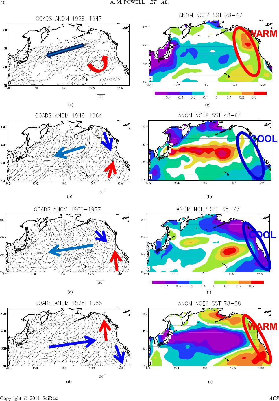

A. M. POWELL ET AL.
40
WARM
(a) (g)
COOL
(b) (h)
COO L
(c) (i)
WARM
(d) (j)

A. M. POWELL ET AL.
41
WA RM
(e) (k)
COOL
(f) (l)
Figure 6. The pattern of the surface wind stress (units: dyn cm–2) and sea surface temperature (units: ˚C) anomalies over the
north Pacific ocean. Left panel: surface wind stress (a) 1928-1947, (b) 1948-1964, (c) 1965-1977, (d) 1978-1988, (e) 1989-1998, (f)
1999-2008; Right panel: sea surface temperature (g) 1928-1947, (h) 1948-1964, (i) 1965-1977, ( j) 1978-1988, (k)1989-1998, (l)
1999-2008.
of water as the impact of El Nino has demonstrated off
the South American coast. El Nino events also affect
upwelling/downwelling, for example, that can have a
marke impact on the fishing off South America. The El
Nino effects are related to the wind and the direction it
blows relative to the shoreline which can cause periods
of upwelling or downwelling that impact the fish popula-
tions. Similarly, changes in the northern hemispheric
wind stress are expected to impact multiple facets of the
ocean current system. What has been demonstrated in
this analysis is the impact of a major atmospheric pattern
change between decadal periods on a core ocean variable
(SST) which in turn can have major ecosystem impacts.
3) Fisheries
The general change in ocean temperature shown in Fig.
6 between the eastern and western Pacific is consistent
with previous research [2,4,5], where the out-of-phase
impacts of SST on the sardine and anchoveta populations
have been demonstrated. Further, Takasuka et al. [3]
indicated that differences in spawning temperatures are a
potential cause of the opposing populations of sardines
and anchoveta in the same regions. While the analysis
offers a possible explanation for the reversal of the sar-
dine and anchoveta populations, a more general conclu-
sion may be possible. If we assume that SST can impact
the fisheries via a variety of pathways (spawning tem-
peratures, food availability via upwelling/downwelling,
etc), then the fish landings should subsequently show
corresponding changes in multiple fish populations.
In Figure 7, the 31 individual species of fish landings
available from NOAA’s Southwest Fisheries Science
Center were analyzed for those that improved or wors-
ened in each regime period. Table 1 identifies the num-
ber plotted for each species of fish shown in Figure 7.
The fish that increased (decreased) in normalized land-
ings were plotted together. A red line was drawn be-
tween those that increased and decreased to help high-
light the impact of the abrup t shifts on the number of fish
species affected. The red line shows the relative change
in biological impact on the ecosystem; in this case, it is
the ecosystem off the California coast (the eastern Pa-
cific). During warm anomaly periods, the number of fish
species with increased normalized landings is greater
than during the cold anomaly periods and vice versa.
While this analysis is for a single region/ecosystem, it is
relevant for understanding the global scale chain of the

A. M. POWELL ET AL.
42
Figure 7. Average normalized fish landing amounts for the U.S. west coast for each species in the periods coincident with
abrupt climate regime shifts. (a) 1928-1947, (b) 1948-2008, (c) 1965-1977, (d) 1978-1988, (e) 1989-1998, (f) 1999-2008. The
X-coordinate number indicates the code for the fish species marked in Table 1. “COOL” and “WARM” indicates the regional
SST anomaly.
events that cause regional ecosystem change. As sur-
mised by Chavez et al. [2], it appears there is a simple
and direct mechanism (atmospheric state change) which
induces wind stress changes impacting the ocean that
result in SST changes (and probably other impacts) that
could affect biological activity regionally.
6. Discussion
The purpose of this paper is to demonstrate that a change
in large scale forcing could produce simple and direct
impacts from the atmosphere to the ocean to ecosystems
to fish landings. These impacts were shown across the
dates of each regime shift identified from a biological
marker (fish landings) and corroborated by other mani-
festations of change in an ecosystem from the literature.
Many factors have been connected with regime shifts.
Ebbesmeyer [16] and Overland et al. [17,18] showed
possible connections with 30 to 100 physical, biological
and climate variables. Collie, et al. [19] pointed out that
smooth, abrupt, and discontinuous shifts can be identi-
fied on the basis of different patterns in the relationship
between the response of an ecosystem variable (typically
biological) and some external forcing. Kim, et al. [20]
demonstrated that specific parameters such as nitrogen
levels, upwelling, and thermocline depth can be associ-

A. M. POWELL ET AL.
43
ated with regime shifts. Aebisher, Coulson and Cole-
brook [21] discussed how temperature and wind stress
variations affect plankton production which can propa-
gate up the food chain and impact fish populations. With
many factors potentially affecting an ecosystem, it
should be obvious that not all fish species will respond
similarly to the same physical change in the environment;
some fish may be affected by specific changes such as
food availability, the depth where the specific fish spe-
cies predominantly lives, spawning temperatures, and
many other factors. Consequently, a specific external
forcing may also be difficult to identify. As a conse-
quence, the analysis approach used the more traditional
atmospheric forcing of the ocean via wind stress as the
general mechanism combined with the simple approach
of looking at how many fish species improved or de-
clined for identifying regime shifts. The results show
clear changes in fish populations across the regime shift
boundaries consistent with large-scale physical forcing
changes - in this case changes in wind stress and sea sur-
face temperature.
The overall chain-of-impacts were shown using a
‘top-down’ logic (from atmosphere to ocean to fish) to
help readers appreciate the traditional linkages between
atmospheric wind and ocean current changes as one
large-scale system acts on another. The global scale
wave amplitude approach provided a method of showing
the abrupt changes in the atmosphere via its relatively
simple pattern of change. The northern hemispheric
wave amplitude is directly related to the wind which im-
pacts the surface wind stress, ocean currents, SST, ad-
vection and upwelling/downwelling. The easiest and
most measured ocean parameter to analyze for this pro-
ject was the SST. The changes in the SST explain the
general pattern of opposing ocean characteristics in the
eastern Pacific versus the western Pacific which could
result in the changes identified by many studies [1-5] in
terms of sardine and anchoveta in the western and east-
ern Pacific for example. Temperature change has been
implicated as a mechanism for the out-of-phase sardine
and anchoveta response through the spawning tempera-
tures which impact survival rates of these two species [3].
However, more than one species of fish should be af-
fected by the abrupt climate shifts and a single species
change may not mark a climate shift. The fish landing
data from NOAA’s Southwest Fisheries Science Center
provided the ability to link the fish population changes
with the abrupt climate shifts and a common ecological
chain via the ocean/ecosystem temperatures. The atmos-
pheric pattern over the Pacific can be generally divided
into two basic patterns which essentially reflect pre-
dominantly wavenumber 1 changes so that when the pat-
tern reverses across a regime shift, regional SST varia-
tions across the Pacific occur synchronously with a cas-
cading effect on the fisheries populations. Figure 8
shows the basic near-surface atmospheric patterns, de-
duced from the COADS analysis, that ap pear to result in
the east-west temperature shifts in the Pacific. These
changes appear to impact the populations of certain spe-
cies of fish. These changes appear to be dominated by
the long easterly or westerly fetches across the Pacific
that set up a specific SST pattern in the Pacific. However,
the Pacific pattern is also influenced by a circular wind
pattern in the southeast Pacific. The southeast Pacific
circular wind pattern can circulate either clockwise or
counter-clockwise and helps generate an SST pattern
similar to the long easterly and westerly fetch wind pat-
terns. This is probably due to unusually strong and
southward displacement of the northern hemispheric
wave pattern in the eastern Pacific.
The net result from this analysis is that northern he-
mispheric wave pattern changes can produce wind stress
changes that generate SST anomalies which in-turn can
affect the fish populations (as determined from the
analysis of the California coastal ecosystem in this study).
The impact of SST change on fisheries populations is
documented in many journal articles. One question that
remains is whether the climate shifts are due to northern
hemispheric wave pattern changes or due to other possi-
ble forcing mechanisms like El Nino.
A discussion of abrupt climate shifts and their impact
on the ocean is not complete without a discussion of El
Nino impacts. El Nino occurs every 5 to 7 years and with
a typical 2-3 year span of intensification which could be
related to nearly every regime shift identified. However,
the pattern of temperature change in the Pacific Ocean is
not consistent with the impact of El Nino but aligned
with mid-to-high latitude atmospheric forcing associated
with the PDO or NAO. The work of Schneider and Cor-
nuelle [22] and Lehodey et al. [6] show convincing evi-
dence that El Nino tends to most impact the equatorial
Pacific and have its impacts described as annual, non-
seasonal and catastrophic while the broader climate im-
pacts are associated with atmospheric forcing are usually
ascribed to the PDO and NAO. The work of Schneider
and Cornuelle [22] use models, observations and statis-
tical analyses to demonstrate the difference in effects
from an El Nino forcing compared to a PDO type at-
mospheric forcing. Their results for the PDO impact re-
gions in the Pacific are in very good agreement with the
patterns shown for this analysis using the COADS data
and the NCDC Extended Reconstructed Sea Surface
Temperatures. Consequently, it supports the contention
the atmospheric-ocean-fisheries impacts shown in this
paper are due primarily to mid-high latitu de atmospheric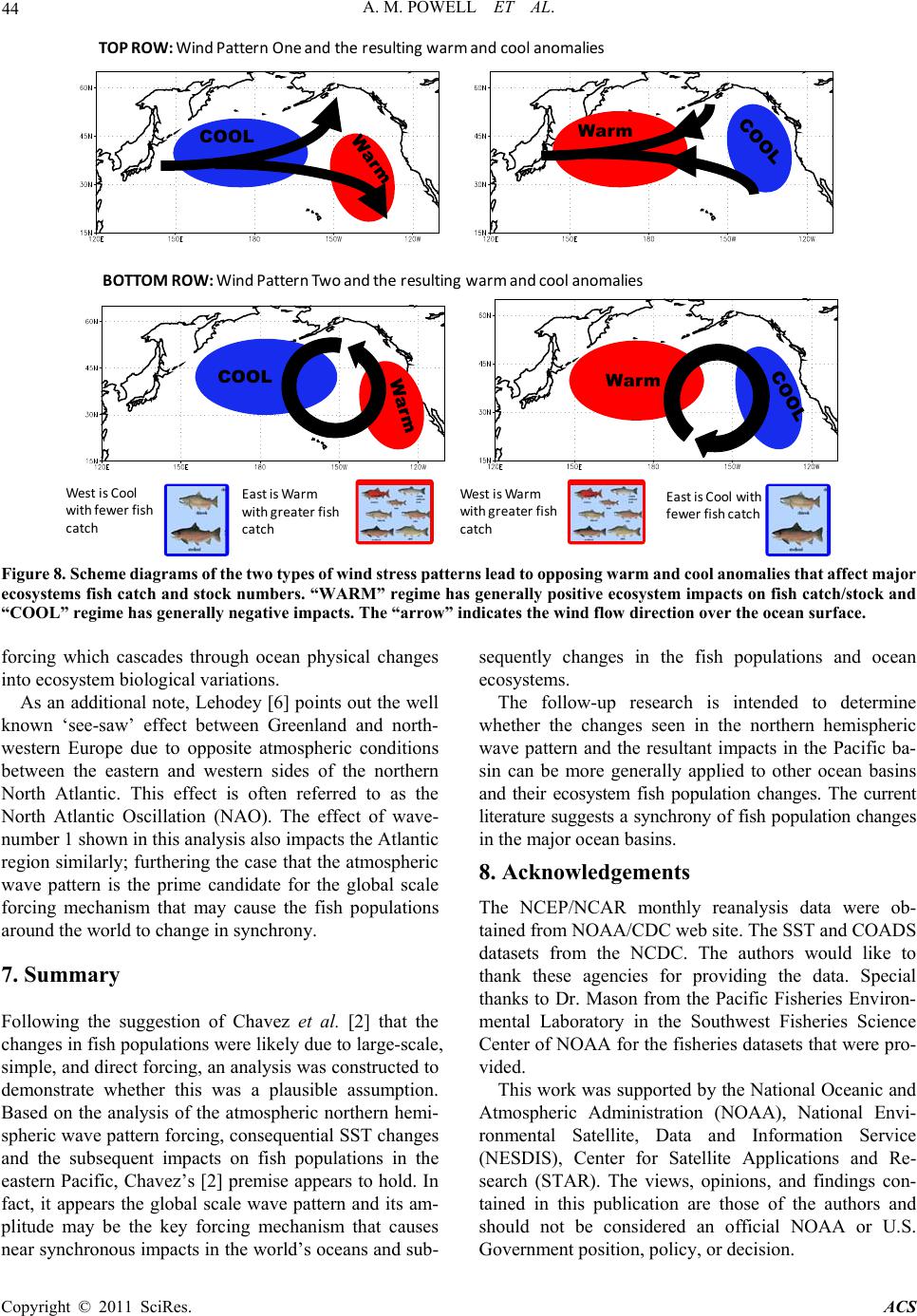

A. M. POWELL ET AL.
44
BOTTOMROW:WindPatternTwoandther esultingwarmandcoolan omalies
COOL
COOL Warm
Warm
TOPROW:WindPatternOneandtheresultingwarmandcoolanomalies
WestisCool
withfewerfish
catch
EastisWarm
with greaterfish
catch
WestisWarm
with greaterfish
catch
EastisC oolwith
fewerfishcatch
Figure 8. Scheme diagrams of the two types of wind stress patterns lead to opposing warm and cool anomalies that affect major
ecosystems fish catch and stock numbers. “WARM” regime has generally positive ecosystem impacts on fish catch/stock and
“COOL” regime has generally negative impacts. The “arrow” indicates the wind flow direction over the ocean surface.
forcing which cascades through ocean physical changes
into ecosystem biological variations.
As an additional no te, Lehodey [6] points out the well
known ‘see-saw’ effect between Greenland and north-
western Europe due to opposite atmospheric conditions
between the eastern and western sides of the northern
North Atlantic. This effect is often referred to as the
North Atlantic Oscillation (NAO). The effect of wave-
number 1 shown in this analysis also impacts the Atlantic
region similarly; furthering the case that the atmospheric
wave pattern is the prime candidate for the global scale
forcing mechanism that may cause the fish populations
around the world to change in synchrony.
7. Summary
Following the suggestion of Chavez et al. [2] that the
changes in fish populatio ns were likely due to large-scale,
simple, and direct forcing, an analysis was constructed to
demonstrate whether this was a plausible assumption.
Based on the analysis of the atmospheric northern hemi-
spheric wave pattern forcing, consequential SST change s
and the subsequent impacts on fish populations in the
eastern Pacific, Chavez’s [2] premise appears to hold. In
fact, it appears the global scale wave pattern and its am-
plitude may be the key forcing mechanism that causes
near synchronous impacts in the world’s oceans and sub-
sequently changes in the fish populations and ocean
ecosystems.
The follow-up research is intended to determine
whether the changes seen in the northern hemispheric
wave pattern and the resultant impacts in the Pacific ba-
sin can be more generally applied to other ocean basins
and their ecosystem fish population changes. The current
literature suggests a synchrony of fish population changes
in the major ocean basins.
8. Acknowledgements
The NCEP/NCAR monthly reanalysis data were ob-
tained from NOAA/CDC web site. The SST and COADS
datasets from the NCDC. The authors would like to
thank these agencies for providing the data. Special
thanks to Dr. Mason from the Pacific Fisheries Environ-
mental Laboratory in the Southwest Fisheries Science
Center of NOAA for the fisheries datasets that were pro-
vided.
This work was su pported by the National Oceanic and
Atmospheric Administration (NOAA), National Envi-
ronmental Satellite, Data and Information Service
(NESDIS), Center for Satellite Applications and Re-
search (STAR). The views, opinions, and findings con-
tained in this publication are those of the authors and
should not be considered an official NOAA or U.S.
Government position, policy, or decision.

A. M. POWELL ET AL.
45
9. References
[1] T. Kawasaki, “Why Do Some Pelagic Fishes Have Wide
Fluctuations in Their Numbers? Biological Basis of
Fluctuation from the Viewpoint of Evolutionary Ecol-
ogy,” FAO Fisheries Report, Vol. 291, 1983, pp.
1065-1080
[2] F. P. Chavez, J. Ryan, S. E. Lluch-Cota and C. M. Ni-
quen, “From Anchovies to Sardines and Back: Multide-
cadal Change in the Pacific Ocean,” Sci enc e, Vol. 299, 10
Jan 2003, pp. 217-221.
doi:10.1126/science.1075880
[3] A. Takasuka, Y. Oozeki, H. Kubota and S. E. Lluch-Cota,
“Contrasting Spawning Temperature Optima: Why Are
Anchovy and Sardine Regime Shifts Synchronous Across
the North Pacific?” Progress in Oceanography, Vol. 77,
2008, pp. 225-232. doi:10.1016/j.pocean.2008.03.008
[4] D. Lluch-Belda, R. A. Schwartzlose, R. Serra, R. Parrish,
T. Kawasaki, D. Hedgecock and R. J. M. Crawford,
“Sardine and Anchovy Regime Fluctuations of Abun-
dance in Four Regions of the World Oceans: A Workshop
Report,” Fisheries Oceanography, Vol. 1, 1992, pp.
339-347. doi:10.1111/j.1365-2419.1992.tb00006.x
[5] B. DeYoung, R. Harris, J. Alheit, G. Beaugrand, N.
Mantua and L. Shannon, “Detecting Regime Shifts in the
Ocean: Data Considerations,” Progress in Oceanography,
Vol. 60, 2004, pp. 143-164.
doi:10.1016/j.pocean.2004.02.017
[6] P. Lehodey, A J. Alheit, B M. Barange, C. T. Baumgart-
ner, D. G. Beaugrand, E. K. Drinkwater, F. J. M. Fro-
mentin, G. S. R. Hare, H. G. Ottersen, F. R. I. Perry, I. C.
Roy, J. C. D. K. Van Der Lingen and F. Werner, “Cli-
mate Variability, Fish, and Fisheries,” Journal of Cli-
mate, Vol. 19, 2006, pp. 1009-1029.
doi:10.1175/JCLI3898.1
[7] Mason, J. E., “Historical Patterns From 74 Years Of
Commercial Landings From California Waters,” Cal-
COFI Rep., Vol. 45, 2004, pp. 180-190.
[8] E. Kalnay, et al., “The NCEP/NCAR 40-Year Reanalysis
Project,” Bulletin of the American Meteorological Society,
Vol. 77, 1996, pp. 437-471.
doi:10.1175/1520-0477(1996)077<0437:TNYRP>2.0.CO
;2
[9] A. M. Powell and J. Xu, “Possible Solar Forcing of In-
terannual and Decadal Stratospheric Planetary Wave
Variability in the Northern Hemisphere: An Observa-
tional Study,” Journal of Atmospheric and So-
lar-Terrestrial Physics, 2011.
doi:10.1016/j.jastp.2011.02.001.
[10] Y. Zhang, J. M. Wallace and D. S. Battisti, “ENSO-like
Interdecadal Variability: 1900-93,” Journal of Climate,
Vol. 10, 1997, pp. 1004-1020.
doi:10.1175/1520-0442(1997)010<1004:ELIV>2.0.CO;2
[11] K. E. Trenberth. and J. W. Hurrell, “Decadal Atmos-
phere-Ocean Variations in the Pacifc,” Climate Dynamics,
Vol. 9, 1994, pp. 303-319.doi:10.1007/BF00204745
[12] W. J. Burroughs, Climate Change a Multidisciplinary
Approach, Cambridge University Press, New York, 2001.
[13] W. J. Burroughs, Weather Cycles Real or Imaginary?
Cambridge University Press, New York. 2003:
[14] W. T. Peterson, , R. C. Hooff, C. A. Morgan, K. L.
Hunter, E. Casillas, and J. W. Ferguson, 2006. Ocean
Conditions and Salmon Survival in the Northern Califor-
nia Current, Web Document.
http://www.nwfsc.noaa.gov/research/divsions/fed/ecosysr
ep.pdf
[15] Hátún, H., M.R. Payne, G. Beaugrand, P.C. Reid, A.B.
Sandø, H. Drange, B. Hansen, J.A. Jacobsen, D. Bloch,
2009: Large bio-geographical shifts in the north-eastern
Atlantic Ocean: From the subpolar gyre, via plankton, to
blue whiting and pilot whales, Progress in Oceanography,
80, 149-162. doi:10.1016/j.pocean.2009.03.001
[16] Ebbesmeyer , C.C., Dr.Cayan, D.R. McLain , F.H. Nichols,
D.H. Peterson and K.T. Redmond, 1991: 1976 step in the
Pacific climate: forty environmental changes between
1968-75 and 1977-1984. In: Proc. 7th Ann. Pacific Cli-
mate Workshop, California Dept of Water Resources, In-
teragency Ecol. Stud. Prog. Report 26.
[17] Overland, J., S. Rodionov, S. Minobe and N. Bond, 2008:
North Pacific Regime shifts: Definitions, issues and re-
cent transitions. Progress in Oceanography, 77, 92-102.
doi:10.1016/j.pocean.2008.03.016
[18] Overland, J. E., J.M. Adams, H.O. Mofjeld, 2000: Chaos
in the North Pacific: spatial modes and temporal irregu-
larity, Progress in Oceanography, 47, 337-354.
doi:10.1016/S0079-6611(00)00041-0
[19] Collie, J.S., K. Richardson, J. H. Steele, 2004: Regime
shifts: can ecological theory illuminate the mechanisms?,
Progress in Oceanography, 60, 281-302.
doi:10.1016/j.pocean.2004.02.013
[20] Kim, H-J, and A.J. Miller, 2007. Did the Thermocline
Deepen in the California Currentafter the 1976/77 Cli-
mate Regime shift?, Journal of Physical Oceanography,
37, 1733-1739. doi:10.1175/JPO3058.1
[21] Aebisher, N. J, Coulson, J. C., & Colebrook, J. M. (1990).
Parallel long-term trendsacross four marine trophic levels
and weather, Nature, 347, 753-755.
doi:10.1038/347753a0
[22] Schneider, N, and B. D. Cornuelle, 2005: The Forcing Of
The Pacific Decadal Oscillation, Journal Of Climate, Vol
18, 4355-4373. doi:10.1175/JCLI3527.1
[23] Mantua, N.J., S.R. Hare, Y. Zhang, J.M. Wallace and R.C.
Francis, June 1997: A Pacific Interdecadal Climate Os-
cillation with Impacts on Salmon Production, Bull. Am.
Meteorol. Soc, 78, 1069-1079.
doi:10.1175/1520-0477(1997)078<1069:APICOW>2.0.C
O;2
[24] Minobe, S., & Mantua, N. (1999). Interdecadal modula-
tion of interannual atmospheric and oceanic variability
over the North Pacific. Progress in Oceanography, 43,
163-192. doi:10.1016/S0079-6611(99)00008-7
[25] Chao, Y; M. Ghil and J.C. McWilliams, 2000: Pacific
Interdecadal Variability in This Century’s Sea Surface
Temperatures, Geophys Res Letters, 27, 2261-2264.

A. M. POWELL ET AL.
46
doi:10.1029/1999GL011324
[26] Hare, S. R., & Mantua, N. J. (2000). Empirical evidence
for North Pacific regime shifts in 1977 and 1989. Pro-
gress in Oceanography, 47, 103-145.
doi:10.1016/S0079-6611(00)00033-1
[27] McFarlane, G.A., J.A. King, R.J. Beamish, 2000: Have
there been recent changes in climate? Ask the fish, Pro-
gress in Oceanography 47, 147-169.
doi:10.1016/S0079-6611(00)00034-3
[28] McPhaden, M.J., and D. Zhang, 2004: Pacific Ocean
Circulation Rebounds, Geophys Res Letters, 31, L18301.
doi:10.1029/2004GL020727
[29] McGowan, J.A., M.J. Cayan, L.M. Dorman, 1998: Cli-
mate-Ocean Variability and Ecosystem Response in the
Northeast Pacific, Science, 281, 210-217.
doi:10.1126/science.281.5374.210
[30] Behrenfeld, M.J., R.T. O’Malley, D.A. Siegel, C.R.
McClain, J.L. Sarmiento, G.C. Feldman, A.J. Milligan,
P.G. Falkowski, R.M. Letelier and E.M. Boss, 7 Decem-
ber 2006: Climate-driven trends in contemporary ocean
productivity, Nature, 144, doi:10.1038/nature05317.
[31] Miller, A.J. and N. Schneider, 2000: Interdecadal climate
regime dynamics in the North Pacific Ocean: theories,
observations and ecosystem impacts. Progress in Ocea-
nography, 47, 355-379.
doi:10.1016/S0079-6611(00)00044-6
[32] Minobe and Shoshiro, 1997: A 50-70 year climatic oscil-
lation over the North Pacific and North America. Geo-
phys. Res. Lett., 24(6), 683-686.
[33] [33] Minobe and Shoshiro, 1999: Resonance in bide-
cadal and pentadecal climate oscillation over the North
Pacific: Role in climatic regime shifts. Geophys. Res.
Lett., 26(7), 855-858.
[34] Stevens, C., S. Levitus, J. Antonov and T.P. Boyer, 2001:
On the Pacific Ocean Regime Shift, Geophys Res Letters,
28, 3721-3724. doi:10.1029/2000GL012813
[35] Minobe and Shoshiro, 2002: Interannual to interdecadal
changes in the Bering Sea and concurrent 1998/99
changes over the North Pacific, Progress in Oceanogra-
phy, 55, 45-64. doi:10.1016/S0079-6611(02)00069-1
[36] McFarlane, G.A, R.J. Beamish, 2001: The re-occurrence
of sardines off British Columbia characterises the dy-
namic nature of regimes, Progress in Oceanography, 49,
151-165. doi:10.1016/S0079-6611(01)00020-9
[37] Beamish, R.J., A.J. Benson, R.M. Sweeting, C.M. Ne-
velle, 2004: Regimes and the history of the major fisher-
ies off Canada’s west coast, Progress in Oceanography,
60, 355-385. doi:10.1016/j.pocean.2004.02.009
[38] Beamish, R.J., R.M. Sweeting and C.M. Nevellie: 2004.
Improvement of Juvenile Pacific Salmon Production in a
Regional Ecosystem after the 1998 Climatic Regime shift,
Transactions of the American Fisheries Society 133:
1163-1175. doi:10.1577/T03-170.1
[39] Beamish,R.J, J. T. Schnute, A. J. Cass, C. M. Neville, and
R. M. Sweeting, 2004: The Influence of Climate on the
Stock and Recruitment of Pink and Sockeye Salmon from
the Fraser River, British Columbia, Canada, Transactions
of the American Fisheries Society 133:1396-1412.
doi:10.1577/T03-221.1
[40] Alheit, J., and M. Niquen, 2004: Regime shifts in the
Humboldt Current ecosystem, Progress in Oceanography,
60, 201-222. doi:10.1016/j.pocean.2004.02.006
[41] Bolt, Jennifer (ed), 2005: Fisheries and the Environment:
Ecosystem Indicators of the North Pacific and Their Im-
plications for the North Pacific and Their Implications for
Stock Assessment, Proceedings of the First Annual
Meeting of the National Marine Fisheries Service’s Eco-
logical Indicators Research Program, Alaskan Fisheries
Service Center (AFSC) Processed Report 2005-04, pgs
103.
[42] Taguchi, B., S-P Xie, H. Mitsudera, A. Kubokawa, 2005:
Response of the Kuroshio Extension to Rossby Waves
Associated with the 1970s Climate Regime Shift in a
High-Resolution Ocean Model, Journal of Climate, 18,
2979-2995. doi:10.1175/JCLI3449.1
[43] Beaugrand, G., 2004: The North Sea regime shift: evi-
dence, causes, mechanisms and consequences, Progress
in Oceanography 60, 245-262.
doi:10.1016/j.pocean.2004.02.018
[44] Brodeur R.D., M. B. Decker, L. Ciannelli, J. E. Purcell, N.
A. Bond, P. J. Stabeno, E. Acuna, G. L. Hunt Jr., 2008:
Rise and fall of jellyfish in the eastern Bering Sea in rela-
tion to climate regime shifts, Progress in Oceanography
77, 103-111. doi:10.1016/j.pocean.2008.03.017
[45] Chiba, S., M. N. Aita, K. Tadokoro, T. Saino, H. Sugisaki,
K. Nakata, 2008: From climate regime shifts to low-
er-trophic level phenology: Synthesis of recent progress
in retrospective studies of the western North Pacific,
Progress in Oceanography, 77, 112-126.
doi:10.1016/j.pocean.2008.03.004
[46] Conners M.E., A.B. Hollowed, E. Brown, 2002: Retro-
spective analysis of Bering Sea bottom trawl surveys: re-
gime shift and ecosystem reorganization, Progress in
Oceanography, 55, 209-222.
doi:10.1016/S0079-6611(02)00079-4
[47] Drinkwater, K.F., 2006: The regime shift of the 1920s
and 1930s in the North Atlantic, Progress in Oceanog-
raphy, 68, 134-151.
[48] Sugimoto, T., S. Kimura, K. Tadokoro, 2001: Impact of
El Nino events and climate regime shift on living re-
sources in the western North Pacific, Progress in
Oceanography 49, 113-127.
doi:10.1016/S0079-6611(01)00018-0
[49] Hollowed, A.B., S. R. Hare, W. S. Wooster, 2001: Pacific
Basin climate variability and patterns of Northeast Pacific
marine fish production, Progress in Oceanography, 49,
257-282. doi:10.1016/S0079-6611(01)00026-X
[50] Rebstock, G.A., and Y. S. Kang, 2003: A comparison of
three marine ecosystems surrounding the Korean penin-
sula: Responses to climate change, Progress in Ocean-
ography 59, 357-379. doi:10.1016/j.pocean.2003.10.002
[51] Seo, H., S. Kim, K. Seong, S. Kang, 2006: Variability in
scale growth rates of chum salmon (Oncorhynchus keta)
in relation to climate changes in the late 1980s, Progress
in Oceanography 68, 205-216.

A. M. POWELL ET AL.
47
[52] Suga, T., A. Kato, K. Hanawa, 2000: North Pacific Trop-
ical Water: its climatology and temporal changes associ-
ated with the climate regime shift in the 1970s, Progress
in Oceanography 47, 223-256.
doi:10.1016/S0079-6611(00)00037-9
[53] Yasunaka, S., Hanawa, K., 2002. Regime shifts found in
the northern hemisphere SST field. Journal of Meteoro-
logical Society of Japan, 80, 119-135.
doi:10.2151/jmsj.80.119
[54] Wong, C.S., Liusen Xie, W. W. Hsieh, 2007: Variations
in nutrients, carbon and other hydrographic parameters
related to the 1976/77 and 1988/89 regime shifts in the
sub- arctic Northeast Pacific, Progress in Oceanography,
75, 326-342. doi:10.1016/j.pocean.2007.08.002
[55] Wooster, W.S., C. I. Zhang, 2004: Regime shifts in the
North Pacific: early indications of the 1976-1977 event,
Progress in Oceanography, 60, 183-200.
doi:10.1016/j.pocean.2004.02.005
[56] Zhang, C.I., J. B. Lee b, Y. I. Seo a, S. C. Yoon, S. Kim:
2004: Variations in the abundance of fisheries resources
and ecosystem structure in the Japan/East Sea, Progress
in Oceanography, 61, 245-265.
doi:10.1016/j.pocean.2004.06.009
[57] Baines, P.G. and C.K. Folland, 2007: Evidence for a
Rapid Global Climate Shift across the Late 1960s, Jour-
nal of Climate, 20, 2721-2744.
doi:10.1175/JCLI4177.1
[58] Frauenfeld, O.W., R.E. Davis, M.E. Mann, 2005: A Dis-
tinctly Interdecadal Signal of Pacific Ocean-Atmosphere
Interaction, Journal of Climate, 18, 1709-1718.
doi:10.1175/JCLI3367.1
[59] Miller, A.J., Daniel R. Cayan, Tim P. Barnett, Nicholas E.
Graham and Josef M. Oberhuber, 1994: The 1976-77
Climate Shift of the Pacific Ocean, Oceanography, 7, No.
1, 21-26
[60] Wu, L., D. E. Lee and Z. Liu, 2005: The 1976/77 North
Pacific Climate Regime Shift: The Role of Subtropical
Ocean Adjustment and Coupled Ocean–Atmosphere
Feedbacks, Journal of Climate, 18, 5125-5140.
doi:10.1175/JCLI3583.1
[61] Ruggerone, G.T., J.L. Nielsen, J. Bumgarner, 2007: Lin-
kages between Alaskan sockeye salmon abundance,
growth at sea, and climate, 1955-2002, Deep-Sea Re-
search II, 54, 2776-2793.
[62] Ladd, C. and LuAnne Thompson, 2002: Decadal Vari-
ability of North Pacific Central Mode Water, Journal of
Physical Oceanography, 32, 2870-2881.
doi:10.1175/1520-0485(2002)032<2870:DVONPC>2.0.
CO;2
[63] Wilderbuer, T.K., A.B. Hollowed, W.J. Ingraham, Jr.,
P.D. Spencer, M.E. Conners, N.A. Bond, G.E. Walters,
2002: Flatfish recruitment response to decadal climatic
variability and ocean conditions in the eastern Bering Sea,
Progress in Oceanography, 55, 235-247.
doi:10.1016/S0079-6611(02)00081-2
[64] Tian, Y., H. Kidokoro, T. Watanabe, 2006: Long-term
changes in the fish community structure from the Tsu-
shima warm current region of the Japan/East Sea with an
emphasis on the impacts of fishing and climate regime
shift over the last four decades, Progress in Oceanogra-
phy, 68, 217-237.