Journal of Applied Mathematics and Physics, 2014, 2, 176-188
Published Online April 2014 in SciRes. http://www.scirp.org/journal/jamp
http://dx.doi.org/10.4236/jamp.2014.25022
How to cite this paper: Wang, J. and Waleffe, F. (2014) The Asymptotic Eigenvalues of First-Order Spectral Differentiation
Matrices. Journal of Applied Mathematics and Physics, 2, 176-188. http://dx.doi.org/10. 4236/ja mp.2014.25022
The Asymptotic Eigenvalues of First-Order
Spectral Differentiation Matrices
Jue Wang1, Fabian Waleffe2
1Department of Mathematics, Union College, Schenectady, USA
2Department of Mathematics, University of Wisconsin-Madison, Madison, USA
Received January 2014
Abstract
We complete and extend the asymptotic analysis of the spectrum of Jacobi Tau
approximations that were first considered by Dubiner. The asymptotic formulas for
Jacobi polynomials
N
P
(,)
,, 1>−
αβ
αβ
are derived and confirmed by numerical approxi-
mations. More accurate results for the slowest decaying mode are obtained. We explain
where the large negative eigenvalues come from. Furthermore, we show that a large
negative eigenvalue of order  appears for
10−< <
α
; there are no large negative
eigenvalues for collocations at Gauss-Lobatto points. The asymptotic results indicate
unstable eigenvalues for
1> α
. The eigenvalues for Legendre polynomials are directly
related to the roots of the spherical Bessel and Hankel functions that are involved in
solving Helmholtz equation inspherical coordinates.
Keywords
Asymptotic Analysis, Spectral Approximations, Jacobi Polynomials, Collocation, Eigenvalue s
1. Introduction
Pseudospectral methods were developed to solve differential equations, where derivatives are computed numer-
ically by multiplying a spectral differentiation matrix [1]. Compared to finite difference methods that use local
information, pseudospectral methods are global, and have exponential rate of convergence and low dissipation
and dispersion errors. However in boundary value problems, they are often subject to stability restrictions [2]. If
the grid is not periodic, the spectral differentiation matrices are typically nonnormal [3], and the nonnormality
may have a big effect on the numerical stability and behavior of the methods. On a grid of size N, pseudos- pec-
tral methods require a time step restriction of
2
()ON
−
[4] for hyperbolic and
4
()ON
−
[5] for parabolic prob-
lems.
Dubiner [6] carried an asymptotic analysis for theone-dimensional wave equation. He pointed out the
( )
ON
boundedness of the eigenvalues of the spectral differentiation matrix with collocation at Legendre points. It was also
proposed in [7] that the
2
()ON
eigenvalues could be shrunk to
( )
ON
byreplacing Chebyshev Tau method with

J. Wang, F. Waleffe
177
Legendre Tau method. That would mean a time step size increase from
2
()
ON
−
to
1
()ON
−
. However, the eigen-
values of Chebyshev and Legend respectral differentiation matrices are extremely sensitive to rounding errors and
other perturbations [4]. On agrid of size
N
, machine rounding could lead to errors of size
2
()ON
. Thus the Le-
gendre Tau method which has an
1
()
ON
−
time step restriction in theory, is subject to an
( )
2
ON
−
restriction in
practice.
The slowest decaying mode and largest wave numbers are often of interest. They affect stabilities and limit time
step sizes of pseudospectral approximations. It is reported in [6] [8] that there exists a large negative eigenvalue of
order
2
N
for Chebyshev spectral differentiation matrix. Where does that eigenvalue come from? When does it ap-
pear? And how does it affect the time step size? In this paper, we will consider the first-order spectral differentiation
matrix and examine the behavior of its eigenvalues asymptotically and numerically.
Let’s consider the first-order eigenvalue problem
( )
, 11,10
du u xu
dx
λ =−<<=
(1)
The spectrum of the differentiation operator is empty. However, the spectrum of the Tau approximations to the
eigenvalue problem affects the stability of the associated wave equation
tx
uu=
on
( 1,1)−
with boundary condi-
tion
( )
1, 0ut=
, whose solution is a leftward translation at speed 1 [3]. Let
()
N
ux
be a polynomial approxima-
tion of degree
N
.
()
N
ux
satisfies
()( )
, 10
N NNN
uDuPx u λ −= =
where
/Dddx≡
,
()
N
Px
is a polynomial of degree
N
. We can write
()( )
x
xs
NN
a
uxeePsds
λλ −
= −∫
for some arbi-
trary constant a. Integration by parts gives
( )( )
()
00
()
1kk
xa
NN
NN
Nkk
kk
DP xDP a
e
ux
λ
λλ
λλ
−
= =
= −
∑∑
. (2)
The non-polynomial contribution (the second term) is eliminated by picking
a=−∞
if
0 λ <R
, and
a= +∞
if
0 λ >R
. We then obtain
( )( )
0
1
k
NN
Nk
k
DP x
ux
λλ
=
=∑
(3)
The boundary condition
( )
10
N
u=
implies
( )
( )
11
0, 0
sN
ePs ds
λ
λ
−
−∞
−=<
∫R
(4)
( )
( )
1
1
0, 0
sN
ePs ds
λ
λ
∞−= >
∫R
(5)
In the Tau method [1], the polynomial approximation
()
N
ux
is determined from the boundary condition
( )
10
N
u=
and the requirement that
()
N
Px
is orthogonal to all polynomials of degree
1n−
with respect to the
weight function
( )
0wx≥
in the interval
( 1,1)−
. For Jacobi weight function
( )()
(,)
1(1 )wxx x
αβ
αβ
=−+
,
( )( )
(,)
NN
Px Px
αβ
=
, the Jacobi polynomial of degree
N
with
,1 αβ >−
.
Assume
0 λ
≠
, otherwise
0 λ
=
corresponds to the trivial solution
( )
0
N
ux=
. From (3), the boundary
condition
( )
10
N
u=
leads to the characteristic polynomial
( )
0
Φ(1)
Nkk
NN
k
DP νν
=
=
∑
, with
1/ νλ =
. It is
proved [9] that the eigenvalues lie in the left half-plane for Jacobi polynomial
( )
(,)
N
Px
αβ
if
11 α
−< ≤
and
1 β >−
. The eigenvalues are computed numerically using the three term recurrence relation for corresponding
Jacobi polynomials [10] (see Figure 1). We will show that the theorem is sharp by obtaining asymptotic results
indicating unstable eigenvalues for
1 α >
.
In order to obtain the asymptotic behavior for large values of
λ
, we use the method of steepest descents to
deform the integration paths to obtain the dominant contribution from saddle points. In general there are two
saddle and two boundary points. The balance between the dominant saddle and boundary contributions leads to
an asymptotic equation for
λ
. The two saddle points collide to form a third-order saddle when
/Ni λ = ±
;
nearly merge when
0 α =
and
/1Ni λ ±
; and are too close to the boundary points when
()ON λ >
.
These cases complicate the analysis.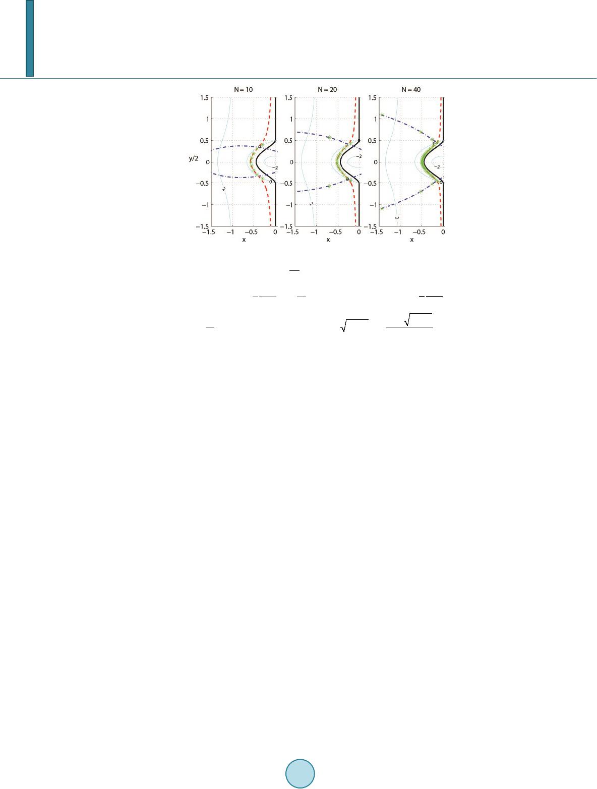

J. Wang, F. Waleffe
178
Figure 1. The limit curve and eigenvalue approximations for Cheby-
shev polynomials (
1
2
αβ
−
= =
). Thick solid:
( )
, 10F µσ =−=
, dash:
( )
3 ln1
,1
2
N
FO
NN
µσ

=−=− −

, dash-dot:
( )
3 ln
,1 2
N
FN µσ == −
1
ON

−

, where
()
2
211
,1 ln
F
σµ
µσµ σµµ

−+

=+ ++



R
.
Thin solid: contours of
()B µ
. Take dash-dot branch for
( )
0B µ >
,
dash for
( )
0B µ <
.
The paper is organized as follows. In Section 2, we present the asymptotic analysis and numerical results for
Chebyshev polynomials. We generalize the results to Jacobi polynomials in Section 3, and derive the approxi-
mations of the slowest decaying mode and largest wave numbers. In Section 4, we show that the eigenvalues for
Legendre polynomials are directly related to the roots of spherical Bessel and Hankel functions. The analysis
and numerical results for collocation methods are explained in Section 5. Finally we conclude in Section 6.
2. Chebyshev Polynomials
We use Chebyshev polynomials
( )( )
NN
Ps Ts≡
to illustrate the approach and derive the asymptotic formulas.
They correspond to the class of Jacobi polynomials with
1/2 αβ == −
and are especially relevant in practice.
With a change of variable
cos s φ =
,
(cos )cos
N
TN φφ =
, and (4) becomes
0coscos( sin)0
ieNd
λφ
π
φ φφ
−
+∞
−=
∫
(6)
It suggests that
N λµ =
. Define
( )
cos i ρφµφ φ =−+
, and
I
twice the above integral,
() 12
02
sin
ii
N
Ied II
ππρφ
π
φφ
+∞ −∞
=+=+
∫∫
(7)
We will apply the method of steepest descent to deform the integration path without changing the value of the
integral, so that it goes through the critical point (saddle point)
*
φ
in such a way that
*
() ρφ R
is maximum
along the path, and
*
() ρφ R
decreases along either direction away from
*
φ
as rapidly as possible. As
N→∞
,
the dominant contributions come from the saddle points and boundary points 0 and
2 π
.
2.1. Saddle Contributions
The saddle points of
( )
ρφ
satisfy the equation
'
( )sinsin0i ρφ µφ = +=
, which implies
*
sin /i φµ = −
. The
steepest-descent curves of
( )
N
e
ρφ
vary as μ varies. We consider two cases:
0 µ ≠R
and
0 µ =R
.
2.1.1.
0≠ µ R
There are two saddle points
()
*
σ
φ
,
()
*
sign 0
σ
σφ = ≠I
, and
()
*
"()0
σ
ρφ ≠
. They satisfy the relationship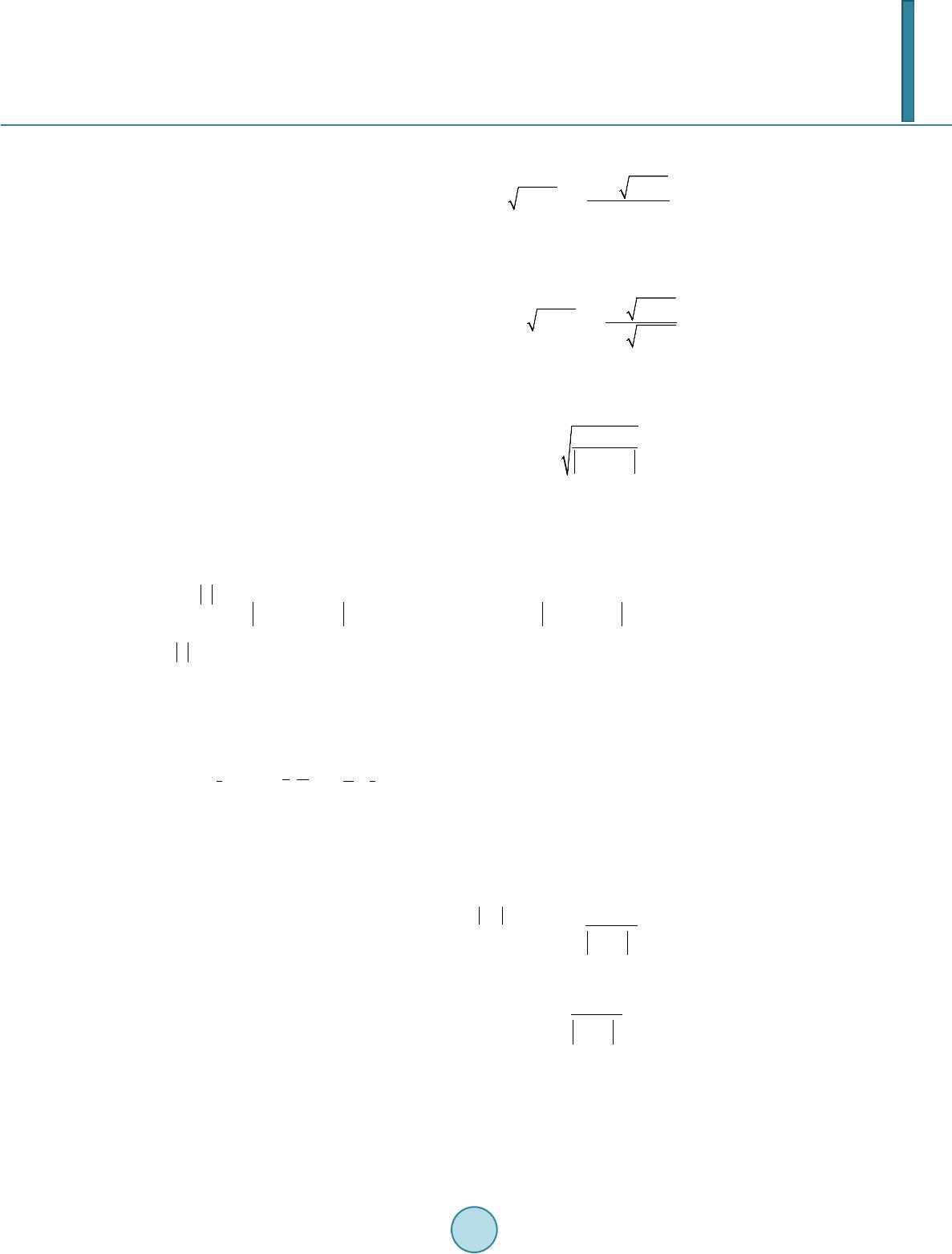

J. Wang, F. Waleffe
179
( 1)(1)
**
φ πφ
−
= −
,
()( )
11
**
( )() ρφ ρφ
−
= −RR
,
()( )
11
**
( )() ρφπ ρφ
−
= −II
, and
( )
( )
()()
2
2
* **
11
cos1 lni
σ σσ
σµ
ρφµ φφσµµ
−+
=−+=++
(8)
The integration paths follow the constant-phase contours
( )
*
()( )
σ
ρφ ρφ =II
, i.e . the steepest-descent curves,
from 0 to
i π +∞
for I1 and from
2 π
to
i π
−∞
for I2, passing through the saddle points
()
*
σ
φ
. The steepest
curves corresponding to the opposite signs of
µ I
are mirror images about
φπ =R
axis. Define
( )
( )
( )
( )
( )
2
11 2
** 2
11
2 1ln11 B
µ
µ ρφρφµµ
−

−+

≡−= ++

++


RR R
(9)
and redefine σ to be
sign ()B σµ =
. Then
*
()
s
I
σ
φ
dominates when
() 0B µ ≠
.
Following the standard saddle point approximation ([11] §7.3), we evaluate the integrals near the saddle
points and obtain the dominant contribution
( )
( )( )
( )
*
() 1/2
**
()
*
2
~sin "( )
N ss i
I INee
σσ
σ
ρφ σθ
σ
π
φφ
ρφ
−
=
( 10)
As
N→∞
when
() 0B µ ≠
.
If
( )
0B µ =
,
( )()
(1)(1)
**
ss s
II I φφ
−
= +
.
2.1.2.
0R µ =
Let
ib µ =
. The two saddles points collide and form athird-order saddle point at
i µ = ±
.
1)
01b<<
. In this case
()
0 B µ <
.
( )
11
*/ 2cosh(1/)ib
φπ
±−
=±−
when
10b−<<
,
1
3/2cosh(1/)
ib π
−
±
when
01b<<
.
( )
( 1)
*
ss
II φ
−
=
.
2)
1b>
. We have
( )
0B µ =
.
( )
11
*sin(1/)b
φ
−
= −
,
( )
11
*sin(1/)b
φπ
−−
=−−
when
1b<−
.
( )
11
*
2sin(1/)b φπ
−
=+−
,
( )
11
*sin(1/)b
φπ
−−
=−−
when
1b>
.
( )
(1)
*
ss
II
φ =
.
3)
1b= ±
.
*
/2b φππ = +
is a third-order saddle point. A similar saddle point approximation leads to
( )
*
11
23
33 2
*
~()6/ 3Γ(1 /3)
bi
i
iN
s
INe ee
ππ π
φ
φ

−
−−


−+
.
2.2. Boundary Contributions
We approximate the contour at
0 φ =
by the straight line
iv φ =
with
[0, ]v ε ∈
and obtain the dominant
contribution at
0 φ =
,
( )
()()()
( )
'
0
0
02
2
'
0
0~~ 0
N
Nv
N b
e
Ieevdv N
ρ ερ
ρ
ρ
−−
−−
∫
( 11)
as
N→∞
. The approximation is the same near
2 φπ =
. Therefore,
( )
( )
( )
0
2
2
'
0(2) ~20
N
bb b
e
II IN
ρ
πρ
−
=+−
(12)
2.3. Balance between Saddle and Boundary Contributions
There are four possible balances from Section 2.1:
1)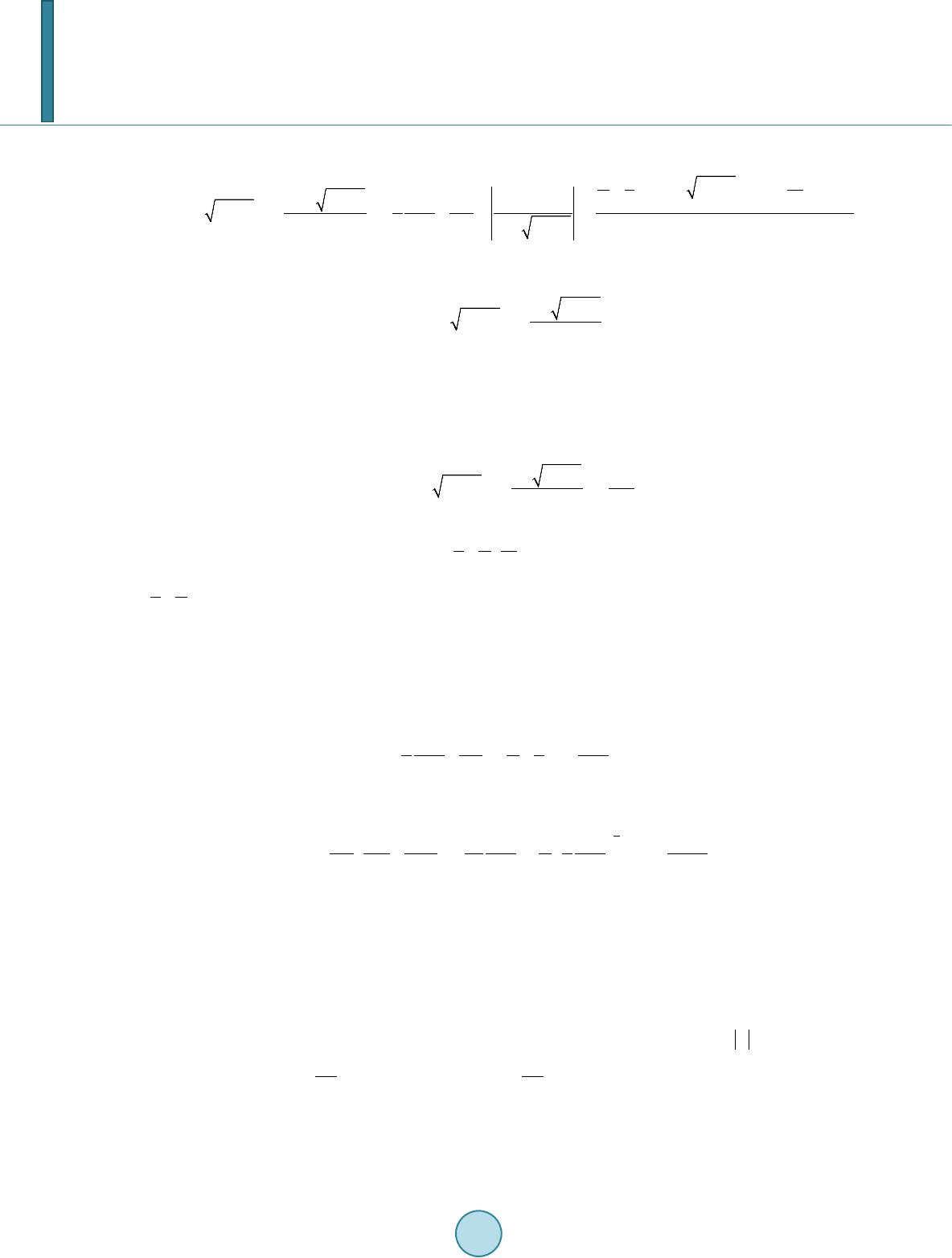
0 µ ≠ R
and
sign ()0B σµ = ≠
, 2)
0 µ =R
and
( )
0B µ =
, 3)
0 µ <R
and
( )
0B µ =
, 4)
0 µ =R
and
( )
0B µ <
.

J. Wang, F. Waleffe
180
In case 1), using
lnln ||arg2zz izki π = ++
,
k∈
, the balance between (10) and (12) leads to
()
2
2
2
22
1arg 1arg2
1 122 3 ln1
1 ln~ln
22
21
ik
Ni
NN N
πσµ π
σµ µ π
µσ µµµµ

−
− −+++

−+ 
+ ++−−−
+
(13)
As
N→∞
, this implies the limit curve
2
2
11
1 ln0
µ
µµ µ

++

−+ +=



R
(14)
In case (2), from Section 2.1.2, the balance leads to the limit curve
0,|| 1 µµ = ≥RI
, i.e. the interval
[, )ii±∞
.
The balances in cases (3) and (4) lead to inconsistent results. The limit curve (14) is in agreement with Dubin-
er’s result ([9] Equation (8.5)). It can be divided into three parts: the interval
[, ) ii±∞
and a curve connecting
i
±
in the left half-plane. The number of eigenvalues distributed around each part is given by the number of in-
tersections of Equation (14) and
2
2
11 2π
1 lnk
N
µ
µµ µ

++

−+ +=



I
(15)
Around
[, )ii±∞
are distributed about
11
22
N
π

−


eigenvalues respectively. There are left about
11
2N π

+


eigenvalues distributed around the curve connecting
i±
in the lefth alf-plane. Figure 1 shows the
limit curve and eigenvalue approximations for Cheybshev polynomials. The numerical eigenvalues are com-
puted using 128-bit or 34 decimal digits of precision. They distribute near the limit curve except a large negative
real eigenvalue
~()ON µ
, which is addressed in the next section. The asymptotic results are accurate even for
small
N
’s.
From Equation (13) we derive that the slowest decaying eigenmode has wave number
3 ln11ln
~lnln 3
2222
NN
bi
NN N
π
µ


−− −±
 


(16)
where
3
2
113127 ln3 ln1
~1/ 1
24282 26ln
NN
bNNN N
πσ σ
π

+
 

−−− ++
 

 

.
The eigenvalues are plotted in Figure 3. They demonstrate better approximations than Dubiner’s results ([6]
Equation (8 .6)).
If the boundary condition
( )
10
N
u−=
is imposed instead, then
0 λ >R
, and the limit curve is a reflection
by the imaginary axis.
2.4. The Large Negative Eigenvalue
The largest wave number limits the time step size of the numerical approximation. When
()ON λ >
, the sad-
dle points
()
11
*
sinh N i φλ
−

=
−

and
( )
21
*
2sinh N i φπ λ
−

= +
−

are too close to the boundaries
00,2
φπ =
.
Thus we have to take the integration path of I1 from 0 up to
( )
1
*
φ
, then to
i π +∞
, and that of I2 from
2 π
up to
( )
2
*
φ
, then to
i π +∞
, going down passing through
( )
1
*
φ
−
to
i π −∞
. Both
( )
1
*
φ
and
( )
2
*
φ
are dominant sad-
dles and
( )
1
*
φ
−
is subdominant. The integral then becomes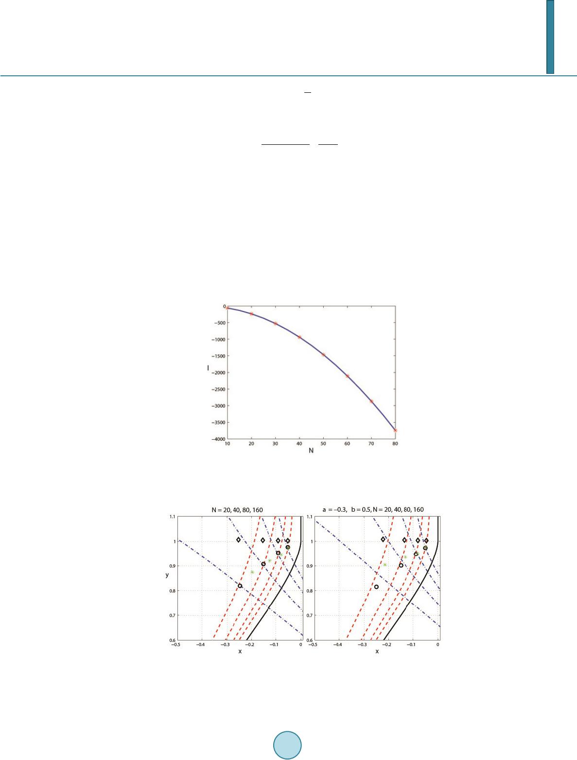

J. Wang, F. Waleffe
181
|| cos|| 12
02
sin
N
i
ii
Ied II
λφφ
ππ λ
π
φφ

+

+∞ −∞
= ++=+
∫∫
(17)
The balance between saddle and boundary contributions implies a polynomial equation for
2
/| |xN
λ
=
,
1
00
!2 (21)!2
nn
nn n
xx
nn n
+
∞
=−=
+
∑
(18)
The real root of (18) approaches a constant as the degree of the equation increases. Solving the equation of
degree 5 gives
2
| |/~N λ
0.5855. This large negative eigenvalue is plotted in Figure 2. The approximation
agrees well with numerical results.
3. Jacobi Polynomials
We now generalize the asymptotic analysis in Section 2 to Jacobipolynomials
( )
(,)
cos
N
P
αβ
φ
with weight func-
tion
()()
cos1cos(1cos) ,,1w
αβ
φφφ αβ = −+>−
.
3.1. Approximation of Jacobi Polynomials
We approximate Jacobi polynomials in two regions, i. e. near 0 and away from 0.
Figure 2. The large negative eigenvalue for Chebyshev
polynomial,
~ λ
0.5855
2
N
, confirmed by numerical
approximations at
N=
[10:10:80], indicated by *.
Figure 3. ○: the slowest decaying eigenmodes for Chebyshevpolynomial giv-
en by (16) (left) and Jacobi polynomialwith
0.3, 0.5 αβ =−=
(right). ◊: Du-
biner’s approximation ([6] Equation (8.6)). *: numerical approximations. The
limit curves move to the rightas N increases.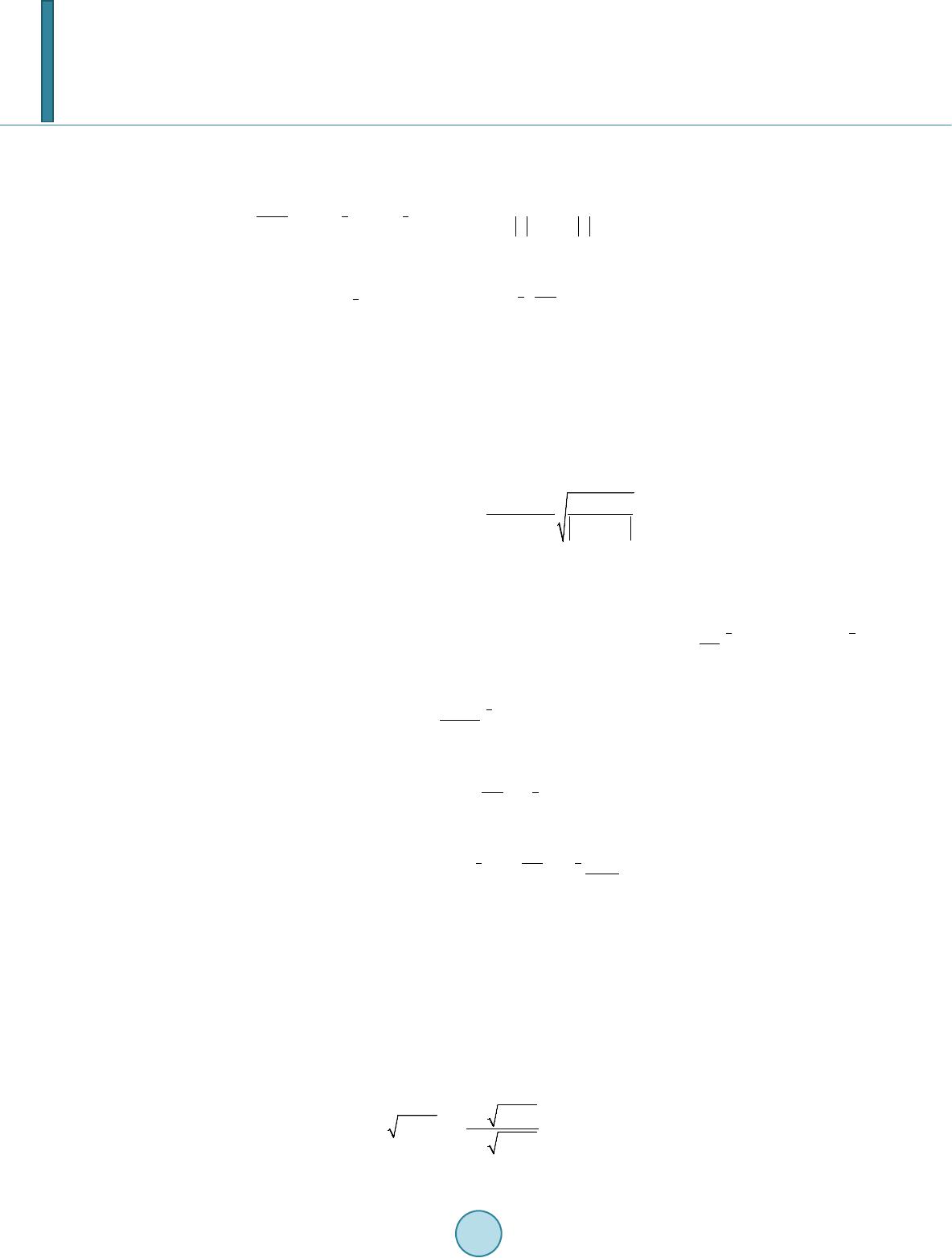

J. Wang, F. Waleffe
182
1) If
||n φ πε −≥
,
( )
( )
,1/2 11
cos~ (2)()()
iNiiN i
N
Pe DeeDe
αβ φ φφφ
φπ
−−− −−

+

(19)
where
( )
111
2 22
2(1 )(1)Dzz z
αβ αβ ++
− ++
= −+
, defined for
1,1z zR<<≤ <∞
,
|| 1
l(m)i zDz
±
→
exists. We de-
rived it from Szego [12] Theorem 12.1.2.
2) If
|0| 1 φ −
,
( )
( )
( )
1
1,22
2
sincos~ (2)2
iN iiNi
N
Peee e
αβ
ααβ φγφγ
φ φπ
−
−
+−−

+

(20)
where
(1/2) /2 γα π =−+
. We derived it from Szego [12] Theorem 12.1.4.
3.2. Limit Curve
Using approximation (19), the integral in (4) becomes
() 1
02
() sin
ii
Ni
IeDed
ππρφ φ
π
φφ
+∞ −∞−−
= +
∫∫
, (21)
with the same
( )
cos i ρφµφ φ =−+
. A similar analysis gives the saddle contribution
( )()
( )
( )
()
*
*
() 1/2 *
()
*
sin 2
~"( )
N
si
i
I NeeDe
σσ
σ
σ
ρφ θ
σ
φ
φπ
ρφ
−
−
(22)
This is in agreement with the results for Chebyshev polynomials in Section 2, where
() ( )
1/2
sin
ii
Dei e
α
φφ
φ
+
−−
=
for
αβ =
.
Using the asymptotic formula for Bessel function of the first kind [13],
( )()
13
22
2
() cos()J zzOz
z
α
γ
π
−
= ++
as
||z→∞
with
( )
arg,0z π δδ ≤− >
, we obtain
( )()
11
2
00
0
2
() cos()J NNON
N
α
φ φγ
πφ
−
= ++
As
N→∞
for
1/3
0
|0|N φ
−
−
. From (20), we have
()
( )( )
1
,22
cos~ 2()
N
PN NJN
αβ α
αβ α
α
φ φφ
−+−
( 23)
Plug (23) to the integral in (4) and we obtain the boundary contribution
31
1
2 22
2
(0) ~2(2)Γ()
bN
I Ne
αβ α
αµ
πα
−−
−−
(24)
(0) ~ 0
b
I
when
0 α =
.
3.2.1.
0
≠ α
The dominant balance is between saddle and boundary contributions. This gives the same limit curve as (14).
The slowest decaying eigenmodes are plotted in Figure 3 for
0.3, 0.5 αβ =−=
.
The theorem in [9] proves that the eigenvalues lie in the left half-plane for Jacobi polynomial
( )
,
N
P
αβ
if
11 α −< ≤
. We have derived asymptotically that the eigenvalue becomes unstable for
1 α
>
.
3.2.2.
0=
α
The dominant balance is between two saddle contributions from
( )
1
*
φ
±
, and this leads to a new limit curve
2
2
2
11
2 1ln0
11
µ
µµ

−+

++ =

++


R
(25)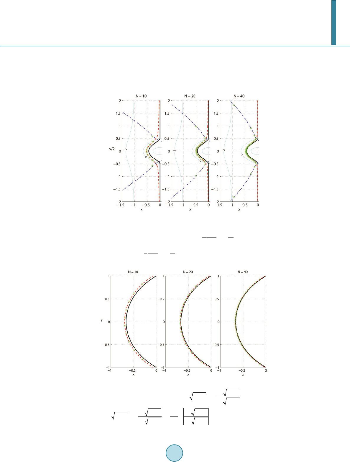

J. Wang, F. Waleffe
183
The intervals
[, )ii±∞
are excluded because only one saddle point contributes.
The limit curve and eigenvalue approximations for Chebyshevpolynomials of the 2nd kind (
1/2 αβ = =
) and
Legendre polynomials (
0 αβ = =
) are plotted in Figures 4 and 5. The eigenvalues huddle around the limit
curve. Note that even at a small
N
= 10, the eigenvalue approximations for Legendre polynomials lie exactly
on the dashed curve, which is true for all the other figures.
Figure 4. The limit curve and eigenvalue approximations for Cheby-
shev polynomials of the 2nd kind (
1/2 αβ = =
). Thick solid:
( )
, 10F µσ =−=
, dash:
( )
1 ln1
,1
2
N
FO
NN
µσ

=−=− −

, dash-dot:
( )
1 ln1
,1 2
N
FO
NN
µσ

==−−


.
Figure 5. The limit curve and eigenvalue approximations for Legendre poly-
nomials (
0 αβ = =
). Thick solid:
2
2
2
11
2 1ln0
11
µ
µµ

−+

++ =

++


R
, dash:
22
2
22
11 11 1
2 1lnln
2
11 11
N
µµ
µµµ

−+ ++

++ =

++ −+


R
.

J. Wang, F. Waleffe
184
3.3. Olver Paths
When
0
α =
and
| |1i µ ±
, the two saddle points
( )
11
*
sin i i φµ
−

= −


and
( )
11
*
sin i
i φπ µ
−−

=−−


nearly
merge. They coincide at
*/2
φπ =
when
i µ = −
, and
3 /2 π
when
i µ =
. The expansions given by the or-
dinary method of steepest descents are not uniformly valid for
| |1i µ ±
. We need to construct uniform ex-
pansions near
i±
and deform the contours into Olver paths [14].
Apply the cubic transformation,
()()
3
1
, ()
3A
ρφµζη µζµ =−+
, to map the saddle points of
( )
ρφ
in the
φ
-plane to the saddle points
η ±
in the
ζ
-plane. It is shown [15] that the mapping is uniformly regular and
one-to-one for all
µ
in a neighborhood of
i±
. The integral (21) becomes
3
1
() 1
3() sins
NA
id
I eDed
d
ζ ηζφ
φ
φζ
ζ
±
−+ −−
=
∫

( 26)
where
±

is a contour running from
−∞
to
/3i
e
π ±
∞
when
1
||iN µ
−
±
, through the saddle point
ζη =
.
The first order approximation gives
5
14 21
26
3333 6
~2Ai2()
iN ii
s
IN eNei
ππ π
π
πµ

−±



±




(27)
for
1
||iN µ
−
±
, where Ai is the Airy function. The eigenvalues are related to the zeros of the Bessel and
Hankel functions of half-integer order
1/2N+
[16]. Further discussions are presented in Section 4.
The slowest decaying eigenmode’s wave number satisfies
( )
21 1
336
Ai2() 0
i
Nei ON
π
µ
±− 
±+ =



. (28)
Ai (z) has a maximal zero
00
,0cc−>
[17]. Then Equation (28) gives
11 2
33 63
0
~2() [(1)]
i
NNecONiNO
π
λµ
−−
=−+ +


. (29)
This is also the largest wave number (see Section 3.4). Hence when
0
α
=
, the largest wave number is of or-
der
N
instead of
2
N
.
3.4. The Large Negative Eigenvalue
The formulas for saddle points contributions are not valid when the saddle points are too close to the boundaries
at
()ON λ >
. The approximation of Jacobi polynomials has to be replaced by Equation (20). If
λ
is not real,
we can take the same integration paths as in Section 3.2 and obtain the saddle contribution. The boundary con-
tribution remains the same with
λ
used first and then replaced by
N µ
. The balance between saddle and
boundary contributions when
0 λ ≠
, or between two saddle contributions when
0 λ
=
gives the same limit
curve as before.
If
λ
is real negative, we take the integration paths as in Section 2.4. The balance leads to a polynomial equ-
ation for
/| |xN λ =
,
2 22
1
0 00
11
cos1sin 0
222 !2!2 (21)
nn
n
nnn
n nn
n xx
cx n nn
n
αα πααπ
+
∞ ∞∞
−
== =
 

− 
 ++−−+=
 
 
 +
 
  


∑ ∑∑
(30)
where
( )
2/221!!
n
ck π = −
when
n
is even
2 nk=
;
2k
n
ck=
when
n
is odd
21nk = +
.
The lowest order approximation by solving Equation (30) of degree 2 gives
2
/ 2cot(/2)cot2(3/ 2)(1/ 2)
~3/2 x
παπ παπαα
α
−+++ −
+
(31)
For
10 α −< <
. Figure 6 shows the ratio
2
/N λ
obtained from (31) and by solving Equation (30) of degree
4, respectively, confirmed by the numerical eigenvalues at
40N=
for different values of
α
. The real root of
the polynomial of degree > 2 is negative for
0 1/2 α <<
and
1/x
approaches
−∞
as
α
approaches 1/2
from the left. Thus, there is a large negative eigenvalue of
2
()ON
for
10 α −< <
and no large negative ei-

J. Wang, F. Waleffe
185
Figure 6. The large negative eigenvalue for
10 α −<<
scaled by
2
N
, compared with the numerical approximations for Jacobipoly-
nomials at
40N=
and
α =
[−0.001, −0. 1: −0.1: −0.9], indicated
as *. Solid: from solving Equation (30) of degree 4, dash: from Equa-
tion (31).
genvalue for
0 1/2 α <≤
. The integral diverges for
1/2 α >
. Therefor there is a large negative eigenvalue of
2
()
ON
for
10
α
−< <
.
When
|0| 1 α −
, the assumption
()ON λ
>
is no longer valid. In this case, the negative eigenvalue is
simply described by the zero of the limit curve given in (14). When
0
α =
, the balance is between two saddle
points. It gives same limit curve as (20). This is not consistent with the assumption
()ON λ >
. So (29) also
gives the largest magnitude eigenvalue which is
()ON
.
4. Legendre Polynomials and Spherical Bessel Functions
Denote Legendre polynomials by
( )
,
NN
PP
αβ
=
,
0 αβ = =
. As indicated in Section 3.3, the eigenvalues are di-
rectly related to the roots of spherical Bessel and Hankel functions.
The emission and scattering of electromagnetic radiation involves solving the vector wave equation [18]. The
solutions are then expressed as an expansion in the orthogonal spherical waves, known as the multipole expan-
sion. Consider the scalar wave equation
2
10 U
Ut
c
∂
∆−=
∂
, where
(,)UU t=x
is the velocity potential,
(,,)xyz=x
and
c
is the speed of sound. For time-harmonic acoustic waves of the form
( )
{ }
,()it U tue
ω −
=xxR
with frequency
0
ω >
, each Fourier harmonic
()ux
satisfies the Helmholtz equation
20u ku∆+ =
where
/kc ω =
is the wave number. It can be rewritten in terms of spherical coordinates
(, ,)r θϕ
. With the expansion
( )
(,)
nn
uf rY θϕ =∑
, the radial function
( )
n
fr
satisfies the equation
2 22
"2' [(1)]0
nn n
rfrfkrn nf+ +−+=
(32)
known as the spherical Bessel differential equation [17] (10.1.1). With a change of variable
( )( )
nn
g rrf r=
,
n
g
satisfies the Bessel differential equation of half integer order
1/2 n+
. Now let
/riz k=
and replace
n
f
by
w
,
n
by
N
, then Equation (32) becomes the modified spherical Bessel equation [17] (10.2.1)
22
"2' [(1)]0z wzwzNNw+ −++=
It has a solution, the modified spherical Bessel function of the third kind [17] (10.2.4),
( )( )
1
2
2
NN
kzK z
z
π
+
=
, where
( )
1
2
N
Kz
+
is the modified Bessel function of the third kind of order
1/2N+
.
Using [17] (9.6.23) and integration by parts
N
times, we obtain

J. Wang, F. Waleffe
186
()( )()
10
1
zszzt
NN N
kzePs dseePtdt
∞∞
− −−
== +
∫∫
Similar to deriving Equation (3),
( )( )
0
1
k
zNN
Nk
k
DP
e
kz zz
−
=
=∑
Thus the eigenvalues
λ
in (3) are the roots of
( )
N
kz
, which are also the roots of Hankel function of order
1/2N+
, spherical and modified spherical Hankel functions using the relations [17] (10.1.1),(10.2.15).
5. Collocation
The Chebyshev collation method and stability analysis was discussed in [2], and then extended to general
Gauss-Radau collocation methods [8] for the one-dimensional wave equation. The Gauss-Radau and Gauss-
Lobatto Jacobi methods were compared and it is shown that the latter is asymptotically stable for
1 αβ ≤≤
[8].
In particular the only Gauss-Lobattoultraspherical method which is marginally stable corresponds to
1 αβ = =
.
We take the discretization
01
11
N
xx x−=< <<=
of the interval [−1,1], and approximate
()ux
by a po-
lynomial
()
N
ux
of degree
N
that satisfies
( )
11
,for,,1 0
N NNN
Duuxxxu λ
−
= ==
(33)
()
N
ux
interpolates the values
01 1
, ,,0
N
aa a
−

at
01
11
N
xx x−=< <<=
and can be written as
( )
1
0()
N
N jj
J
uxal x
−
=
=
∑
, where
{ }
()
j
lx
are the cardinal functions. Substituting
N
u
into (33) gives the matrix
system with eigenvalue
λ
. Collocation at zeros of orthogonal polynomials (Gauss points) is identical to the
Tau method with Gauss quadrature. We consider three sets of Gauss-Lobattopoints
11
[, ]
T
N
xx
−
=x
:
1) Chebyshev extreme points:
cos
j
j
xN
π
= −
; 2) Chebyshev extreme points of the 2nd kind:
j
xj=
th zero of
'
N
U
; 3) Legendre extreme points:
j
xj=
th zero of
'
N
P
.
They can all be described as zeros of
'( )
N
Qx
, where
N
Q
is Chebyshev, Chebyshev of the 2nd kind and Le-
gendre polynomial of degree
N
, respectively. Defineresidual
()
() ()
NN
RxDu x λ = −
. It is a polynomial of
degree
N
that vanishes at
1x=−
and zeros of
'( )
N
Qx
. Thus N
R
takes the form
()
(1)'( )
NN
RxxQx = +
. In
general, for Jacobi polynomial
( )
,
N
P
αβ
, from [19],
( )()
( )
()( )
( )
,1, 1
1
1
1 11
2
NN N
d
RxxPNxP
dx
αβα β
αβ
++
−
= +=++++
Using (19) and (20), we obtain approximations of
( )
cos
N
R φ
for
φ
away from 0 and near 0. The balance
remains valid with
()()( )
colcol col
2
2, 1,1
1
ii
i
D eDe
e
φφ
φα αββ
= =+=+
+
However, for Legendre extreme points, the balance is now between saddle and boundary contributions since
col 1
α =
, and the limit curve is the same as the other two. Figure 7 shows the eigenvalues obtained using the
Tau and collocation methods, together with their limit curves for Chebyshev (
1/2 αβ == −
), Chebyshev of the
2nd kind (
1/2 αβ = =
) and Legendre (
0 αβ = =
) polynomials. Collocations at Chebyshev and Legendre ex-
treme points are stable. Collocation at Chebyshev extreme points of the 2nd kind becomes unstable. In general,
collocation at Gauss-Lobatto points is stable when
11
α +≤
, i.e.
0 α ≤
, unstable when
0 α >
. There is no
large negative eigenvalue with Chebyshev extreme points used. This can be derived asymptotically using the
same method as before, or simply follows from
col 1
αα = +
.
6. Conclusions
We have presented pseudospectral approximations of the first-order spectral differentiation matrices with zero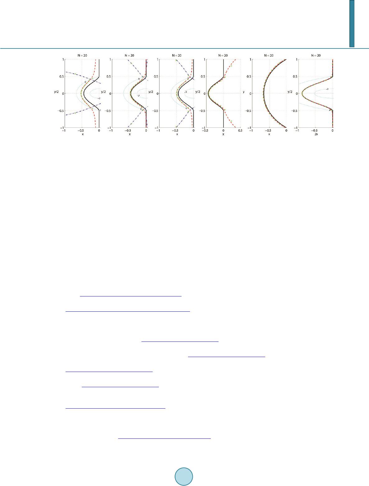

J. Wang, F. Waleffe
187
Figure 7. From left to right: Tau method at
1/2 αβ ==−
, collocation at Chebyshev extreme points, Tau method at
1/2 αβ = =
, collocation at Chebyshev extreme pointsof the 2nd kind, Tau method at
0 αβ = =
, collocation at Legendre
extreme points.
boundary condition. We use the method of steepest descent to deform the integration path without changing the
value of the integral, in order to obtain the dominant contributions from saddle and boundary points. This ap-
proach leads to the asymptotic formulas for the eigenvalues of Jacobi Tau method. Numerical examples with
Chebyshev of the 1st and 2nd kind and Legendre polynomials are presented. They agree well with the asymptotic
analysis, even at small sizes.
The approximations for the slowest decaying modes give more accuracy than those obtained in [6]. The larg-
est wave numbers have raised interest in stabilities in pseudospectral approximations. We show that a large neg-
ative eigenvalue of order
2
N
appears for
10 α
−< <
. The collocation methods are also examined. There are
no large negative eigenvalues for collocations at Gauss-Lobatto points.
For Jacobi polynomials, the eigenvalues lie in the left half-plane if
11 α
−< ≤
. We show that the theorem is
sharp by obtaining asymptotic results that indicate unstable eigenvalues for
1 α >
. The eigenvalues for Legen-
dre polynomials are related to the roots of Bessel and Hankel functions of half-integer order, spherical and mod-
ified spherical Bessel and Hankel functions. These results complete Dubiner’s earlier analysis [6].
References
[1] Canuto, C., Hussaini, M.Y., Quarteroni, A. and Zang, T.A. (1988) Spectral Methods in Fluid Dynamics. Springer, New
York. http://dx.doi.org/10.1007/978-3-642-84108-8
[2] Gottlieb, D. (1981) The Stability of Pseudospectral Chebyshev Methods. Mathematics of Computation, 36, 107-118.
http://dx.doi.org/10.1090/S0025-5718-1981-0595045-1
[3] Trefethen, L.N. and Embree, M. (2005) Spectra and Pseudospectra: The Behavior of Nonnormal Matrices and Opera-
tors. Princeton University Press.
[4] Trefethen, L.N. and Trummer, M.R. (1987) An Instability Phenomenon in Spectral Methods. SIAM Journal on Nu-
merical Analysis, 24, 1008-1023. http://dx.doi.org/10.1137/0724066
[5] Weideman, J.A.C. and Trefethen, L.N. (1988) The Eigenvalues of Second-Order Spectral Differentiation Matrices.
SIAM Journal on Numerical Analysis, 25, 1279-1298. http://dx.doi.org/10.1137/0725072
[6] Dubiner, M. (1987) Asymptotic Analysis of Spectral Methods. Journal of Scientific Computing, 2, 3-31.
http://dx.doi.org/10.1007/BF01061510
[7] Tal-Ezer, H. (1986) Spectral Methods in Time for Hyperbolic Equations. SIAM Journal on Numerical Analysis, 23,
11-26. http://dx.doi.org/10.1137/0723002
[8] Jackiewicz, Z. and Welfert, B.D. (2003) Stability of Gauss-RadauPseudospectral Approximations of the
One-Dimensional Wave Equation. Journal of Scientific Computing, 18, 287-313.
http://dx.doi.org/10.1023/A:1021121008091
[9] Csordas, G., Charalambides, M. and Waleffe, F. (2005) A New Property of a Class of Jacobi Polynomials. Proceedings
of the AMS, 133, 3351-3560.
[10] Weideman, J.A.C. and Reddy, S.C. (2000) A Matlab Differentiation MatrixSuite. ACM Transactions on Mathematical
Software, 26, 465-519. http://dx.doi.org/10.1145/365723.365727
[11] Arfken, G.B. and Weber, H.J. (1995) Mathematical Methods for Physicists. Academic Press.

J. Wang, F. Waleffe
188
[12] Szego, G. (1939) Orthogonal Polynomials. AMS Colloquium Publication, 23.
[13] Waston, G.N. (1995) A Treatise on the Theory of Bessel Functions. 2nd Edition, Cambridge University Press.
[14] Olver, F.W.J. (1970) Why Steepest Descents? SIAM Review, 12, 228-247. http://dx.doi.org/10.1137/1012044
[15] Chester, C., Friedman, B. and Urse l l, F. (1957) An Extension of The Method of Steepest Descents. Proc. Cambridge
Philos. Soc., 53, 599-611. http://dx.doi.org/10.1017/S0305004100032655
[16] Driver, K.A. and Temme, N.M. (1999) Zero and Pole Distribution of Diagonal Padé Approximants to the Exponential
Function. Questiones Mathematicae, 22, 7-17. http://dx.doi.org/10.1080/16073606.1999.9632055
[17] Abramowitz, M. and Stegun, I.A. (Eds.) (1965) Handbook of Mathematical Functions: With Formulas, Graphs, and
Mathematical Tables. Dover Publications.
[18] Colton, D. and Kress, R. (1998) Inverse Acoustic and Electromagnetic Scattering Theory. 2nd Edition, Springer.
http://dx.doi.org/10.1007/978-3-662-03537-5
[19] Doha, E.H. (2002) On the Coefficients of Eifferentiated Expansions and Derivatives of Jacobi Polynomials. J. Phys. A:
Math. Gen., 35, 3467-3478. http://dx.doi.org/10.1088/0305-4470/35/15/308