Journal of Applied Mathematics and Physics, 2014, 2, 131-137
Published Online April 2014 in SciRes. http://www.scirp.org/journal/jamp
http://dx.doi.org/10.4236/jamp.2014.25017
How to cite this paper: Denis-Vidal, L., et al. (2014) Parameter Identifiability and Parameter Estimation of a Diesel Engine
Combustion Model. Journal of Applied Mathematics and Physics, 2, 131-137. http://dx.doi.org/10.4236/jamp.2014.25017
Parameter Identifiability and Parameter
Estimation of a Diesel Engine Combustion
Model
Lilianne Denis-Vidal*, Zohra Cherfi, Vincent Talon, El Hassane Brahmi
University of Technologie of Compiègne France, LMAC , ROBERVAL Compiègne, France
Received Dec emb er 2013
Abstract
In this paper an original method based on the link between a piecewise identifiability analysis and
a piecewise numerical estimation is presented for estimating parameters of a phenomenological
diesel engine combustion model. This model is used for design, validation and pre-tuning of en-
gine control laws. A cascade algebro-differential elimination method is used for studying identi-
fiability. This investigation is done by using input-output-parameter relationship. Then these re-
lations are transformed by using iterated integration. They are combined with an original numer-
ical derivative estimation based on distribution theory which gives explicit point-wise derivative
estimation formulas for each given order. Then new approximate relations, linking block of para-
meters and outputs (without derivative) are obtained. These relations are linear relatively to the
blocks of parameters and yield a first estimation of parameters which is used as initial guess for a
local optimization method (least square method and a local search genetic algorithm).
Keywords
Calib r ati on, Genetic Algorithms, Global Optimization, Identifia bility , Identification Algorithms,
Internal Combustion Engines
1. Introduction
The use of model to predict system behavior in order to make technical choices or to understand its functioning
has become very important during the last decade. This is particularly true in automotive industry, especially
because of the increase of emissions constraints and the will to optimize fuel consumption. A phenomenological
model has been used. Such models have the main advantage to be quite simple and directly linked with observa-
ble phenomenon. In this paper a Wiebe double phase combustion model is proposed and investigated. On the
other hand their use is effective only if they were beforehand calibrated.
The main advantage of this mathematical model is its execution speed. Thus, it helps to carry out real-time
simulations as for HIL (Hardware In the Loop). But its lack of physics makes impossible any form of explora-
*Corresponding author.

L. Denis-Vidal et al.
132
tion out of its training zone. Some of its parameters must be estimated [1].
Before performing parameters estimation, it is necessary to investigate their identifiability. Identifiability
falls into the category of inverse problem. It is a priory question: do two distinct parameters give distinct
output?
In case of negative answer, one will not be able to estimate it except by some additional a priori knowledge:
the model has to be reconsidered. There are three main approaches for studying identifiability of controlled and
uncontrolled non linear dynamical systems described by differential systems. The first one is based on equiva-
lence theory [2,3], the second one considers the Taylor series expansion [4], and the last one comes from elimi-
nation theory [5]. This last theory gives a possible procedure for estimating parameters without any information
about them. Few studies use it efficiently [6 ]. The differential elimination method necessitates model with
smooth function which is not the case of our model and more some output derivatives of high order may be es-
timated. A piecewise differential elimination is proposed in order to take into account the non smooth func-
tions which appear in our model. Then it is shown how the resulting calculus can be used to build a parameter
estimation procedure for this type of model.
The paper is organized as follows. In the second section the phenomenological model is presented as well as
the resulting mathematical system. The third section is devoted to identifiability: some definitions are recalled,
piecewise identifiability tests and results are given. The fourth section treats the transformation of the relations
obtained from identifiability previous study. Section 5 is devoted to numerical procedure: the numerical estima-
tion of derivatives and the resulting estimation procedure and numerical results are given. Finally, conclusions
are drawn in the last section.
2. The Diesel Combustion Model
2.1. The Phenomenological Model
The Wiebe model with double phases facilitates the modeling of traditional diesel combustions. It is based on
first thermodynamics principle. The internal energy variation follows the equation:
/
ii
dUddQdWh dm θ =++
∑
wit h
U: internal energy [J],
θ
: crankshaft degree, dQ: energy exchange with outside [J/s], dW: work with outside
[J/ s]
h
i
: specific enthalpy [J/kg],
dm
i
: mass flow with outside [kg/s]
In the case of the combustion chamber we can identify:
• The energy exchanges with outside are equal to losses on the walls and the contribution of combustion ener-
gy.
• T he work is the one of the piston on gases.
• The exchanges of matters are mass flows through the exhaust and intake valves.
The Wiebe phases represent the combustion of pre mixture and diffusion. These two combustions succeed one
another during one engine cycle. Below we describe shortly process of diesel combustion.
After the intake and gas compression, fuel is introduced into the combustion chamber. This fuel is believed in
vapor form in the case of Wiebe. The compression overheats the fuel. This heating will cause its ignition. This
starts the two flames of combustion of pre mixture and diffusion.
The first phase represents the flame of pre mixture: at this stage, air and fuel are perfectly mixed. When the
time of ignition is reached, a mass combustion occurs. At this stage there is a multitude of points of ignition in the
combustion chamber. We say that the combustion is controlled by chemistry.
The second phase represents the diffusion flame: in this case chemistry becomes infinitely fast because of the
rise of temperature due to the pre mixture flame. The combustion is then controlled by the speed of fusion of the
air and the fuel. That is why we call it diffusion flame.
The Wiebe model thus makes possible to model these two flames. We need to associate to this model of heat
release, additionally work of the piston on gases and the exchanges with the walls:
• Work is in traditional form—P.dV, where P is the pressure in the chamber and dV is the volume variation.
• Exchanges with the walls are in form
w
h.S.(T-T)
, where H, S,T and
T
w
are respectively, the coefficient of

L. Denis-Vidal et al.
133
exchange, the surface of exchange, the temperature of gases in the combustion chamber and the temperature
of the walls.
With internal energy (U) and mass (M) in the chamber, we can calculate pressure and temperature of gases.
This temperature is calculated with the first law of Joules U = CnMT
with Cn = heat capacity for constant volume [J/kg/K], T = temperature [K].
The pressure is calculated with the law of perfect gases:
P(MrT) /V)=
where, P = pressure [Pa], r = perfect gases constant [J/kg/K] and V = volume [m3].
2.2. Mathematical Model
This model can be described in state space form as follows
S(p, ) ν
:
/(,, )()dXdF XpC θθ νθ = +
,
00
and (),(,)XX YhX θθ = =
Using the notations of the previous subsection, this system is explained as follows.
X denotes the state vector in the model described in the previous section, X = (M,U) ’, Y denotes the output
and Y = X in our problem,
[0, ] θ ∈Θ
, p = (p
1
,….,p
l
) denotes the vector of parameters, each parameter is a
positive number. In the case of the phenomological model the vector of parameters is given by:
pp
P (,fpre,,mp,,md)
pd
α = ∆∆
and
ν
is a square wave input,
max( ()()QinjH ADVHADVinj ν θθ =−−− −
with Qinjmax > 0 and
inj
0 θ >
,
adΩ
denotes the set of
such inputs. H is the well known Heaviside function:
()1 if 0 and ()0 if 0Hx xHxx=>=<
Putting:
• C = (1, Ccarb, Tcarb -Lvap)’, F = (F1, F2)’, with:
F1(X,, p)0 θ =
and
( )
pp
F2(X,, p)k1XQparois (, X) (fpre)f1(p,)H(ADVp ))(1fpre)f2(p,) H(ADVd)) θαθθθ θ = −+−+−−
whe r e
•
( )()
k1X(1)(U / V(dV / d) γθ =−−
is a known function,
γ
is the constant of adiabatic compression
• K = PCI.M inj, PCI and Minj are known constants,
f1(p, ) θ
and
f2(p, ) θ
are the derivatives relatively to
θ
of
1 111
pd
Exp[(/) ( ADVp)] et Exp[(/) (ADVd)]
mpmpmd md
pd αθ αθ
+ +++
−∆ −−∆−
•
( )
pp pp
Qparoi(,X)Sp k2X αα =
where Sp is a known constant. and k2(X) is a known function and
pp
α
is a
parameter to be identified.
In this model, we assume that:
H1: 0ADVADVpADVd< <<<Θ
and H2: k2(X) not equal to 0.
3. Ident ifia bil ity
3.1. Definitions
Now some useful definitions are recalled. In the following the vector of parameter is denoted p = (p1,…pl)
Definition1
The parameter pi is said to be globally identifiable if, for any (ph,pt) and pih not equal to pit there exists an
input such that the systems
S(ph, ) ν
and
S(pt, )
ν
yield different outputs.
Definition2
The model is said to be globally identifiable if all parameters are globally identifiable.
3.2. Identifiability Analysis
In this section, an identifiability study is proposed by using piecewise relations linking successive known func-
tions and parameters. The main identifiability results are given in the following.
Theorem1 The diesel combustion model
S(p, ) ν
is globally identifiable.
This result is a consequence of the following proposition.
Propo sitio n1 I np ut-output-parameter relations are given successively by:
1) If
[ [
0, ADV θ ∈

L. Denis-Vidal et al.
134
12
(,)k(U (,))Sk(M(,),U(,))
pp p
dU p ppp
d
θθαθθ
θ
−= −
(ES1)
2) If
]ADV, ADV[
pd
θ ∈
22
2 111 11
11
22
[( )]()[]
ppprepp pre
yyy yy
yADVmyfADVm f
θθ
θθ θ
θθ
∂∂∂ ∂∂
−−=− −−+
∂∂ ∂
∂∂
(ES2)
()()
121
1z1
p
pp pre
m
p
ym yf
α
θθ
+
−
∂
−=+ +
∂∆
(ES3)
3) If
]ADV ,min(,ADV)[
d inj
θθ ∈ Θ+
2
2
222
22
2
[()] (1)]()(1)
pred dpre
yyy
y fADVmyf
θ
θθ
θ
∂∂ ∂
−+ −−−=−−−
∂∂
∂
(ES4)
242
1
z(m1)( yf1)
d
dd pre
m
d
y α
θθ
+
− ∂
−=++−
∂∆
(ES5)
where:
()( )()
112 max
yM,U,pUSkM,UQ( CTL)
pppinjpcarb carbvap
dU K
d
α
θ
− =−−−−
( )( )
21 1
yM,U,pyM,U,pKff(p,)
pre
ωθ −=+
()
( )
24
z(,p)and z
pd
mm
pd
ADV ADV θθ θ −=− =−
For the proof of this proposition a piecewise differential elimination is performed and successively input-
output parameters relations are obtained and then global identifiability of parameters and model.
4. Iterated Integration, Input-Output-Parameter Relations and Derivatives
Estimation
The main objective of this paper is to give an efficient procedure for a numerical estimation of parameters. This
procedure begins with input-o utput -parameter relations. Often these relations require the knowledge of deriva-
tives of observed signal. The observations are noisy and estimation of derivatives becomes an ill posed problem.
In order to overcome this problem, this paper proposes a new computation algorithm for determining the para-
meters with noisy observed signal. This algorithm is based on two steps described in next sections.
4.1. Iterated Integration and Input-Output-Parameter Relations
The first step consists in integrating as far as possible the input-output-parameters relations in order to remove
derivatives and by using integration by parts and iterated integrals using the well known C auchy’s formula:
1
()
....()()( 1)!
xt xi
aa a
xt
dtfu duftdt
i
−
−
=−
∫∫ ∫
,
This leads to inte gr o-differential relations which are used to build our estimation procedure. However, in
these relations, some first order derivatives remain. Then, derivatives have to be estimated. This approach has
been developed in [6].
4.2. A Method for Estimating Derivatives
Description of the method
For estimating the derivatives an original method is given in [6]. It is based on distribution theory and the

L. Denis-Vidal et al.
135
main tools are the test functions which are infinitely differentiable functions with compact support.
In this paper the test functions are deduced from the following function with support in [−1;1],
2
1
1
1
()
01
x
ex
x
x
ψ
−

<
=
≥



A translation and a dilatation allow obtaining an infinitely differentiable function
I
ε
ψ
with a support in-
cluded in a given interval
.I
ε
They play the role of sliding windows. The method is based on the combination
of a truncated Taylor expansion of the signal and test functions. The use of the truncated Taylor expansion for
the derivatives estimation is classical (finite difference, etc...).
The difference is the way to use it. Let us consider y an analytic function in the interval [a,b]
IR⊂
. Such that
the length of
I
ε
is
2 ε
the truncated Taylor expansion yN of y is an approximation of y. It is given by:
( )
() 0
0
0
()
() !
n
Nn
N
yy
n
θθ
θθ
−
=
∑
and then
( ) ( )
()()0
0
()
()()!
nk
N
kn
Nk
nk
yy E
nk
θθ
θθ
−
=
−
=−
∑
for k = 0….N.
Multiplying this equality by
I
ε
ψ
and integrating on
I
ε
, because the support of
I
ε
ψ
is included in
I
ε
and
by using integration by part, the following linear system triangular is obtained
()
() ()
0
()1() ()
Nk
nk
nkN I
nk I
yytt dt
ε
ε
θα ψ
−
=
= −
∑∫
for k= 0….N. (Ss)
The unknown are
() 0
()
k
y θ
for k = 0….N, and the determinant of the system is
0
N
α
which is not equal to
zero. Then
() 0
()
k
y θ
for k= 0….N can be obtained as solution of this system. Replacing
yN
by y in (Ss) a
numerical estimation
( )
,0
kN
y
ε
θ
of
() 0
y()
k
θ
is obtained.
Error due to the noise on the signal
In [7], the authors bring out two kinds of perturbations. The first ones, like the constant perturbations whose
amplitude is unknown are said structured. They can be annihilated by linear differential operators and it is, for
example, the case of a random noise whose mean is constant and unknown. The second ones are said unstruc-
tured and correspond to a high frequency perturbation which can be reduced by low pass filters like iterative in-
tegrals. Thus, any noise can be written as the sum of such noises. The method based on the distribution theory
allows annihilating a part of the structured noises. On the other hand the integration reduces the effect of un-
structured noise which corresponds to high frequency perturbations.
5. Methods for Estimating Wiebe Model Parameters and Numerical Results
In numerical study, the cylinder pressure P has been used instead of the internal energy U because the observed
data in our possession are those of the cylinder pressure P.
5.1. Description of the Methods
Two methods have been set up. Each method consists in 2 steps. The first one is the same for both approaches.
Estimation and inte gro -differential equations
This first step is based on successive global optimizations which are made on successive intervals.
Firstly we focus on the parameter
pp
P (,fpre,,mp,,md)
pd
α = ∆∆
. The exact observation, corresponding to
the exa ct value of p, is more or less perturbed by noise. So, integro differential equations are not satisfied by the
noisy output. Moreover, the observation is not carried out at any time and the data are a set of measures:
k,mes(tk,pex) k, for k 1...qPP ε =+=
k ε
, for each k, is assumed to be a normal random noise with zero mean. Each integro-differential equation
corresponds to an integro-differential polynomial. The outputs are noisy, and are carried at each discretization
time tk for each polynomial and the derivatives are estimated, therefore a least square minimization problem is
performed. This step gives us a first estimation. But the crankshaft degree interval: [ADVp,ADVd] is small and
the number of discretization points is also small. Consequently the estimations of some integrals are not accurate
enough and then, some parameters are not well estimated: the pressure reconstruction is not satisfactory. This
fact leads us to implement local optimization methods to improve the accuracy. The first estimation obtained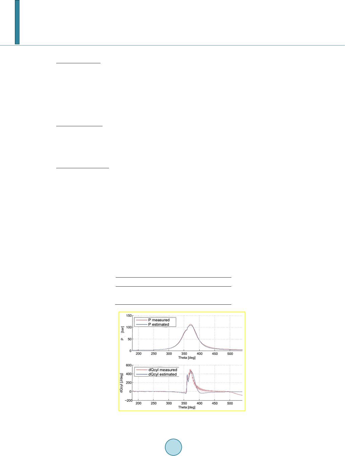

L. Denis-Vidal et al.
136
with this first step can be used as initial guess for a local optimization. In the following it is denoted p0.
Local optimization
Having studied sensitive analysis, we noticed that the thermodynamic quantity
dQcyl / d θ
is sensitive to
some parameters while the pressure is less. This makes necessary the joint use of these two quantities.
More, the cylinder pressure P and the heat release
dQcyl / d θ
are two thermodynamic quantities of different
nature. In order to perform the local optimization, the system
S(p, ) ν
is used and not input output integro-dif-
ferential equations. The first step of the methods doesn’t allow the use of the heat release: this quantity don’t ap-
pear in the input-output relations. These two thermodynamic quantities can be used for local optimization by
considering an augmented system with the classical link between cylinder pressure and heat release.
Now, we will describe precisely the step 2 corresponding to each of the two methods.
First method, step 2
The objective function considered in this second step for the first method is the function J:
112 2()(, )(, )J pwFpwFp θθ = +
where wi are weights, F1 and F2 are respectively the least square residual
corresponding respectively to the pressure and to the heat release.
The Levenberg Marquardt has been used in order to solve the minimization problem: find p which minimize J
with initial guess p0 given by the first step.
Second method, step 2
The previous objective function is a weighted sum. Because of a lack of information on the physical pheno-
menon, a relevant choice for the weights is difficult. In order to overcome this problem a multi-objective opti-
mization is considered in the second method. NSGA-II algorithm [8] has been used for solving the minimization
problem find p which minimize J2, with s and p taken in a domain around p0.
5.2. Numerical Results
In this section, numerical results by using these two methods, denoted GM + L.M for the first one and GM +
NSGA. II for the second one, are presented and compared.
The first method gives accurate results: relative error is small, however the second one give best results for
the accuracy. On the other hand, the first one is the best for the computation time. The genetic algorithm used by
the second one computes 3 × N × M times the value objective function, where M is the population size and N
the number of iterations. The following table presents the relative error for the reconstruction of experimental
curves. In Figure 1 and Fig ure 2 experimental and reconstructed pressure and heat release are given for each
methods.
method (e.r) pour P (e.r) pour dQcyl
GM + L.M 0.0021 0.13
GM+NSGA.II 0.0011 0.069
Figure 1. Pressure and heat release reconstruction: GM+LM.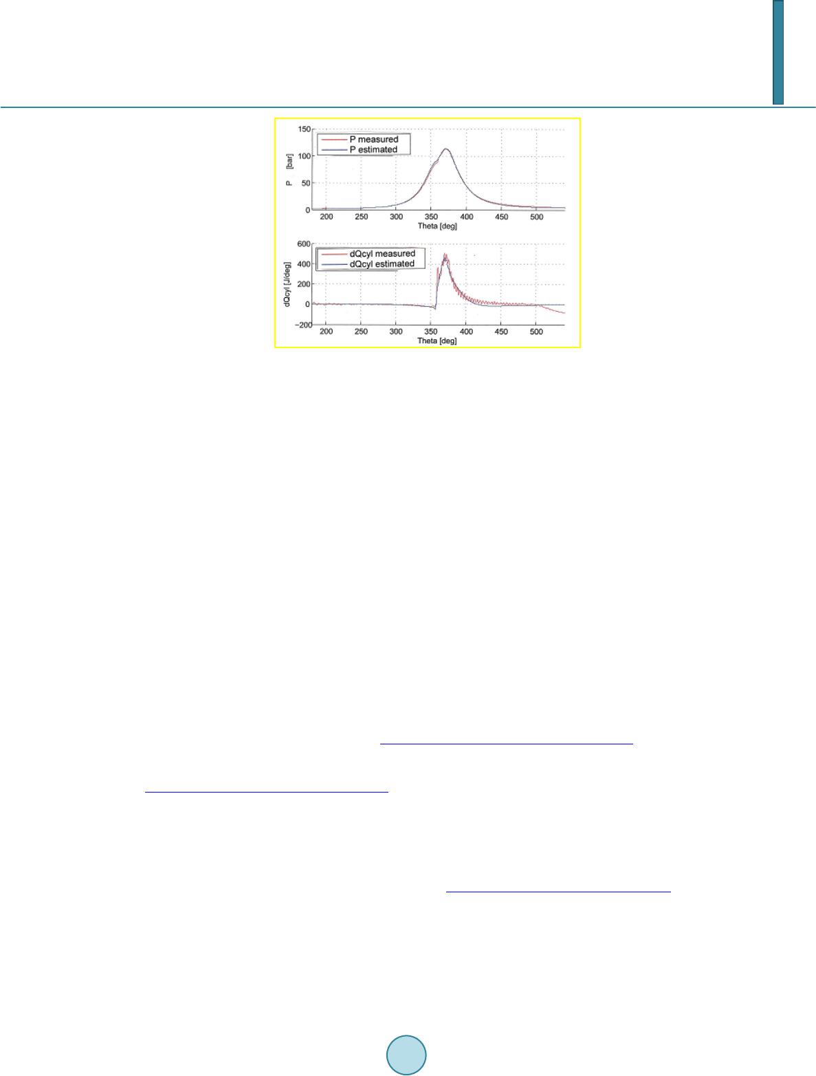

L. Denis-Vidal et al.
137
Figure 2. Pressure and heat release reconstruction: GM +
NSGA.II.
The best reconstruction particularly for the heat release is given by the second method, and more, this method
is less sensitive to the first estimation than the first one.
6. Conclusion
In this paper an approach for analyze identifiability of the Wiebe model combustion with double phases has
been proposed. The input-outp ut-parameter relations which come from the identifiability study have been origi-
nally exploited in order to perform the parameters estimation step. These relations contain some derivatives of
the noisy observations. Estimation of higher derivatives from noisy data is a numerical ill-posed problem. In or-
der to overcome this problem, successive integrations as far as possible have been done and combined, for the
remaining derivatives, with an efficient new method for estimating derivatives. This method is based on distri-
bution approach and for the first time, it is applied to an industrial problem. This approach allows decreasing the
order of derivatives and then to estimate remaining derivatives of low order efficiently with a new method which
play the role of noise filter. Then, this estimation is used as initial guess for a local optimization algorithm and a
multi-objective optimization algorithm in order to improve parameter estimation results. This methodology has
shown its efficiency and the resulting solutions lead to a good reconstruction of the actual observations.
References
[1] Tal o n , V. (20 04 ) Modélisation 0-1D des moteurs à allumage commandé. Ph.D Thesis, Orléan University, Orléan.
[2] Deni s-V id al , L. and Joly-Blanchard , G. (2004) Equivalence and Identifiability Analysis of Uncontrolled Nonlinear
Dynamical Systems. Automatica, 40, 287-292. http://dx.doi.org/10.1016/j.automatica.2003.09.013
[3] V ajda, S., Godfrey, K.R. and Rabitz, H. (1987 ) Similarity Transformation Approach to Identifiability Analysis of Non-
linear Compartmental-Models. Mathematical Biosciences, 93, 217 -248.
http://dx.doi.org/10.1016/0025-5564(89)90024-2
[4] Pohjanpalo, H. (19 78) System Identifiability Based on the Power Series Expansion of the Solution. Mathematical Bio-
sciences, 41, 21-33.
[5] Ollivier, M. (1990) Le problème de l'identifiabilité structurelle globale: Approche théorique, méthodes effectives et
bornes de complexité. Ph.D Thesis, Ecole Polytechnique, Paris.
[6] V erdièr e, N., Denis-V id al , L. and Joly-Blan chard , G. (2012) A New Method for Estimating Derivatives Based on a
Distribution Approach. Numerical Algorithms, 61, 163 -18 6. http://dx.doi.org/10.1007/s11075-012-9535-4
[7] Fliess, M., Mboup, M., Mounier, H. and Sira-Ramirez, H. (2005) Questioning Some Paradigms of Signal Processing via
Concrete Examples. Proc. Summer School: Fast Estimation Method in Automatic Control and Signal Processing, Pari s.
[8] Deb , K. and Agrawal , R .W. (1995) Simulated Binary Crossover for Continuous Search Space. Complex Systems, 9,
115-148.