Journal of Applied Mathematics and Physics, 2014, 2, 124-130
Published Online April 2014 in SciRes. http://www.scirp.org/journal/jamp
http://dx.doi.org/10.4236/jamp.2014.25016
How to cite this paper: El-Fayez, F.M.N. (2014) My Limiting Behavior of MHD Flow with Hall Current, Due to a Porous
Stretching Sheet. Journal of Applied Mathematics and Physics, 2, 124-130. http://dx.doi.org/10.4236/j amp .2014. 25016
Limiting Behavior of MHD Flow with Hall
Current, Due to a Porous Stretching Sheet
Faiza M. N. El-Fayez
Department of Mathematics, Princess Nora Bint Abdul Rahman University, Riyadh, KSA
Received December 2013
Abstract
An electrically conducting fluid is driven by a stretching sheet, in the presence of a magnetic field
that is strong enough to produce significant Hall current. The sheet is porous, allowing mass
transfer through suction or injection. The limiting behavior of the flow is studied, as the magnetic
field strength grows indefinitely. The flow variables are properly scaled, and uniformly valid as-
ymptotic expansions of the velocity components are obtained through parameter straining. The
leading order approximations show sinusoidal behavior that is decaying exponentially, as we
move away from the surface. The two-term expansions of the surface shear stress components, as
well as the far field inflow speed, compare well with the corresponding finite difference solutions;
even at moderate magnetic fields.
Keywords
MHD Flow, Hall Current, Stretching Sheet, Porous Sheet, Limiting Behavior
1. Introduction
The flow due to a moving surface is an important field of fluid mechanics. It has several applications; for exam-
ple, in production of glass and paper sheets, drawing of plastic films, and extrusion of metals and polymers.
Crane [1] obtained an exact solution for the two-dimensional flow of a Newtonian fluid due to a linearly
stretching sheet. The velocity components in this case has simple forms; tending to their limits monotonically in
an exponential manner as we move away from the surface. The simplicity of this solution invited several authors
to consider different related problems, which exhibit the same behavior; e.g. [2]-[8].
One such problem is when the fluid is electrically conducting and a magnetic field is applied normally to the
surface. For weak magnetic fields, the flow remains two-dimensional and a closed-form solution is still possible
to attain. The Lorentz force acts to restrain the flow; causing faster exponential tendency to the limits. When the
magnetic field is strong enough to produce significant Hall current, the problem changes considerably. It be-
comes three-dimensional. The Hall current is associated with an electromagnetic force which derives a trans-
verse flow. A closed-form solution is no longer possible.
It is interesting to explore the nature of this MHD flow in the presence of Hall current. To that end, the limit-
ing behavior of the flow as the magnetic field grows indefinitely is studied. The straightforward perturbation
analysis leads to secular behavior, which is removed by parameter straining [9]. Three-term uniformly valid asy-

F. M. N. El-Fayez
125
mptotic expansions are, thus, obtained. The presence of the Hall current leads to an exponential tendency to the
limits of sinusoidal nature. The flow involves alternating regions of forward and backward velocity components.
Finite difference solutions are also obtained and show qualitative adherence to the predicted limiting behavior
even for moderate magnetic fields. Quantitatively, the two term expansions show excellent agreement with the
numerical results.
2. Formulation of the Problem
A totally ionized fluid is driven by an insulated sheet, which is symmetrically stretching with speed us that is
proportional to the distance x from the axis of symmetry z. Specifically, us =
ω x, where ω is a constant of pro-
portionality. The sheet is porous; allowing a uniform fluid injection of speed ws in the z direction. Otherwise, the
fluid would have been quiescent. A uniform magnetic field is applied in the z-direction. The magnetic Reynolds
number is small, so that the induced magnetic field can be neglected; and the applied field maintains its uniform
magnetic flux density B. On the other hand, the magnetic field is strong enough to produce significant curvature
in the electrons trajectories; leading to considerable Hall current [10].
The fluid is incompressible of density
ρ , viscosity µ , electrical conductivity σ , Hall coefficient h (=1/ene);
where ne is the number density for the electrons and -e is the electron charge. All these parameters are consi-
dered constant.
The velocity components: u in the x-direction, v in the transverse y-direction, and w in the z-direction, as well
as the pressure p are dependent on x and z only. They are governed by the following continuity and Navier-
Stokes equations, which include components of the Lorentz force corrected for the Hall current,
0
xz
uw+=
(1a)
2
2
()[]( )
1
xzxx zzx
σB
ρuu wuμuupu mv
m
+=+ −−−
+
(1b)
2
2
()[]( )
1
xzxx zz
σB
ρuvwvμvvv mu
m
+ =+−+
+
(1c)
()[ ]
xzxx zzz
ρuw wwμww p+ =+−
(1d)
where subscripts denote differentiation, m = σ hB is the Hall parameter. Note that m may be positive or negative
in accordance with the sign of B; i.e. depending on whether the magnetic field is directed away from or toward
the sheet. However, as a simultaneous change of the signs of m and v leaves the problem unaltered, only
non-negative values of m need to be considered.
At the surface, z = 0, the adherence conditions u = ω x and v = 0 apply; together with the injection condition w
= ws. Far from the sheet, as z~∞, the fluid has pressure p∞ and velocity components u~0 and v~0.
The problem admits the similarity transformations z = (
µ / ρω )½ ζ , u = ω xF( ζ ), v = ω xG( ζ ), w = ( ωµ / ρ )½H( ζ ),
and p = p∞+
ωµ Q( ζ ); leading to the following problem.
0HF
′+=
(2a)
2
ˆˆ ˆ
( )0FHF FβnF mG
′′ ′
− −−−=
(2b)
ˆˆ ˆ
( )0GHGFG βnG mF
′′ ′
− −−+=
(2c)
Q HHH
′ ′′′
= −
(2 d)
0 :1,0,
s
F GHH ζ == ==
(2e-g)
~:~0, ~0, ~0FGQ ζ ∞
(2h-j)
where
2
( ,,1)
ˆˆ ˆ
(,,) 1
m
mn m
β
β =
+
, with
2
σB
β
ρω
=
being the magnetic interaction number; and a dash denotes differ-
rentiation with respect to ζ .

F. M. N. El-Fayez
126
3. Asymptotic Analysis
We are interested in the limiting behavior of the flow as β ~∞ with fixed m; i.e. as
ˆ
β
~∞ with fixed
ˆ
m
and
ˆ
n
.
That F (0) = 1 irrespective of the value of
ˆ
β
means that F =
O
(
ˆ
β
0). The leading term in Equation (2b) is
ˆ
β
ˆ
n
F. It can be balanced by the diffusion term
F′′
in a contracting region in which z =
O
(
ˆ
β
−1/2). Then, Equa-
tion (2a) gives H =
O
(
ˆ
β
−1/2); consistent with which Hs must be
O
(
ˆ
β
−1/2). Consequently, Equation (2d) gives
Q =
O
(
ˆ
β
0). In Equation (2c), the driving force for the transverse flow is the Hall effect expressed by
ˆ
β
ˆ
m
F.
This requires
G′′
~
ˆ
β
ˆ
m
F; leading to G =
O
(
ˆ
β
0).
New stretched variables
1/2 1/2
,
ˆ ˆ
β βVH ζη = =
(3a,b)
are introduced; transforming Problem (2) to the form
0 VF
′+=
(4a)
-1 2
ˆ
ˆ ˆ()FnF mGβVF F ′′ ′
−+ =+
(4b)
-1
ˆ
ˆ ˆ()GnG mFβVG FG
′′ ′
−− =+
(4c)
-1
ˆ
QV βVV
′ ′′′
= −
(4d)
( )( )( )
0 1,00,0
s
F GVV= ==
(4e-g)
()( )( )
~0, ~0,~0FGQ ∞∞∞
(4h-j)
where, now, the dashes denote differentiation with respect to η .
We expand the flow variables in powers of
ˆ
β
−1 in the form
-1 -2
012
ˆ ˆ
~ZZ βZβZ++ +
(5)
where Z stands for F, G, V, and Q. The problems for Zn, n = 0,1,2,3,···, are lin.ear. For Z0, we get the basic flow
solutions
0
F
=EC,
0
G
= −ES,
22
0s
[()]/( )VV αEαCγSαγ=+− +−+
, and
0
Q
= −EC, where α and γ satisfy
α
2 −
γ
2 =
n
ˆ
and 2 αγ =
m
ˆ
; with S = sin γη , C = cos γη and E = exp(− αη ), for short. For Z1, the solutions in-
volve secular terms of the form η ES and η EC, the removal of which is effected by straining the parameters
ˆ
m
and
ˆ
n
in the form (5); and the procedure can be continued to higher orders.
The following expansions up to
O
(
ˆ
β
−2) are obtained
2 2-1-2
01
ˆ ˆ
ˆ~( )nαγβ αvβ αv−++ +
(6a)
-1 -2
01
ˆ ˆ
ˆ~2mαγβ γvβ γv+++
(6b )
-12-22 3
1112 2
ˆ ˆ
~[()] [()()]F ECβECfSgEfβE CfSgE cECaSb++−+++++ +
(6c)
-12-22 3
1112 2
ˆ ˆ
~[()][()()]GES βECgSfEgβECgSfE cECaSb−+− −+−++++

 
(6d)
-1 2
011 1111
-22 3
22 222
ˆ
~[(S)][{()()}/ 2]
ˆ ˆ
ˆ
[{()()}/ 2()]
Vv λEγ αCβvλEγgαfSαgγfEfα
βvλECγgαfSαgγfEc αE CaSb
C+ −+++++−−+
+++− ++++
(6e)
where symbols appearing on the right-hand sides are given in Appendix.
Of interest are the longitudinal and transverse components of the shear stress at the surface, as well as the far-
field speed. They are represented, respectively, by
-1 -2
112 2
ˆ ˆ
(0)~()(2 3)Fβfgβf gcab αα γαγααγ
′−+++ − +−−+ +

(7a)
-1 -2
112 2
ˆ ˆ
(0)~()(2 3)Gβgfβg fc ab γα γαγααγ
′−+−+−−− − ++

 
(7b)
-1 -2
012
ˆ ˆ
( )~VvβvβvV
∞
∞ +++=
(7c)
The expansion for the pressure can be obtained from
-1 22
1
2ˆ()QFβVV
∞
=−+ −
(7d )

F. M. N. El-Fayez
127
which is the result of integrating Equation (4d) and the use of Equation (4a) and Condition (4j). This is not given
here for brevity.
The above expansions describe how the flow behaves as
β ~∞ with fixed m. They reveal a sinusoidal behavior
that dies out exponentially as we move away from the surface. This behavior is solely due to the Hall effect,
which is also responsible for the presence of the transverse velocity component G. When the Hall current is ne-
glected; i. e. m = 0, Expansion (6b) leads to
γ = 0, Expansion (6d) gives G = 0, Expansions (6c) and (6e) reduce
to F = E and
s
(1)/VV E α =+−
, respectively, while Expansion (6a) translates to α satisfying
2-1s
ˆ(1) 1
βV αα −=+
. These results coincide with the exact solutions of the degenerate cases of Gupta and Gup-
ta [2] and Andersson [3].
Expansions (6) describe the limiting case when
β ~∞ with m =
O
( β
1/2), as well. All we need is to set
γ = α . It
should, however, be noted that, now, as
ˆ
β
=
O
( β
1/2), the stretching (3) is weaker; being
O
( β
1/4). Moreover,
the perturbations to the basic flow proceed in powers of
β
−1/2.
4. Results and Discussion
The asymptotic expansions obtained above are tested against corresponding numerical results. The problem de-
scribed by Equation (4) is solved numerically in double precision, using Keller’s two-point, second-order-accu-
rate, finite-difference scheme [11]. A uniform step size ∆
η = 0.01 is used on a finite domain 0≤ η ≤ η
∞. The
value of
η
∞ is chosen sufficiently large in order to insure the asymptotic satisfaction of the farfield conditions
(4h,j). (As pointed out by Pantokratoras [12], a small value of
η
∞ can lead to erroneous results.) The non-linear
terms are quasi-linearized, and an iterative procedure is implemented; terminating when the maximum errors in
F′
(0),
G′
(0), and H(∞) become less than 10−10.
The numerical results exhibit the attenuating sinusoidal behavior predicted by the asymptotic analysis. This is
clearly illustrated in Fig. 1 showing the longitudinal and transverse velocity profiles F(
η ) and G( η ), when β = 20,
m = 10, Vs = 20, and
η
∞ = 500. However, at such low value of
β , a fixed period of oscillation is not sustained.
When
β is increased to100 the F and G profiles, respec tiv ely, cross the zero line first at η ≈ 7.79 and 15.44 then
at
η ≈ 23.15 and 30.87; thus sustain ing the same period τ ≈ 30.8. The two profiles cross the zero line several
times later, but with much smaller magnitudes; maintaining the same period, though.
How quantitatively useful the asymptotic expansions of the previous section can be, is next investigated. To
generate numerical values, for given β , m and Vs, we need to determine the coefficients α , γ , λ , v0, f1, g1, v1…, etc.
To that end, we use Expansions (6a) and (6b) and the pertinent equations of Appendix A to obtain expansions of
these coefficients in the form (5). In particular, the coefficients of the expansions which are involved to
O
(
ˆ
β
−1)
are found to be
22 1/21/2
01ˆˆˆ
[ {()}]
2
αnmn= ++
,
00
ˆ/2γmα=
,
2 21
0 00
()λαγ
−
= +
,
00s0 0
vVλ α= −
,
1 00
1
2
αv= −
,
Figure 1. Velocity profiles; β = 20, m = 10, Vs = 20.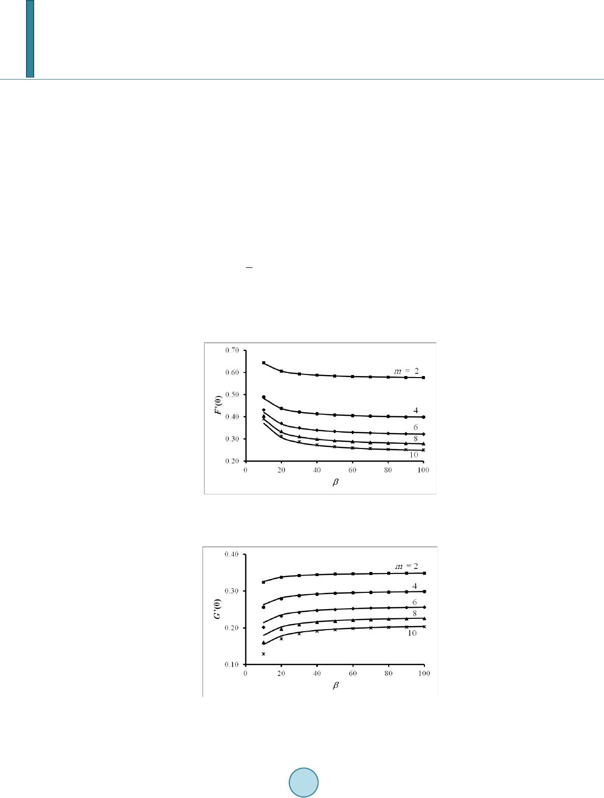

F. M. N. El-Fayez
128
1
0γ=
,
2
100 101
2( )λλααγ γ=−+
,
010110
()vλαλα=−+
,
10000 1023
fλ γ(γθα θ)/θ=−+
,
100 00 1023
gλ γ(α θγθ)/θ= −
,
and
10010100
ˆ ˆ2vλ(nfmg) /α=−+
; where
22
1 00
3θα γ= +
,
2
ˆ
θm=
, and
22
312
θ θ θ= +
. The following expansions
are also obtained
1 2
010 10010
ˆ ˆ
(0)) ( )
-
Fαβ (ααfγgβ
−
+
′=−+ −++O
(8a)
1 2
01010010
ˆ ˆ
(0)) ()
-
Gγβ (γα gγfβ− +
′=−+ −+−O
(8b)
2-1
000110
ˆ
()()( )Vvβvv β
−
∞= +++O
(8 c )
Results of the two-term asymptotic expansions (i.e., up to
O
(
ˆ
β
-1) )are proved to be in close agreement with
the numerical results, even at values of β as low as 20. This is illustrated in Figures 2 and 3 for
F′
(0) and
G′
(0) with different values of m, and in Figure 4 for V(∞) with different values of Vs.
The period of the sinusoidal oscillations
τ = 2 π / γ takes the form
22 1/21/22
1ˆ
ˆ ˆˆˆ 4 [{()}]/()
2
τπ nmnm β− = +++O
(9)
For m = 2, 4, 6, 8, 10 Equation (9) gives
τ = 17.87, 20.73, 23.97, 26.96, 29.68, respectively, which are close to
the corresponding numerically predicted values
τ ≈ 17.86, 20.75, 24.01, 27.01, 29.76 obtained with β = 100 and
Vs = 0. That is,
τ is independent of Vs to
O
(
ˆ
β
−2), is also tested numerically. Varying Vs between −10 and 10,
with
β = 100 and m = 1, gives τ = 19.54 ± 0.04, as compared to the asymptotic value τ ≈ 19.53.
Figure 2. Longitudinal surface shear
(0)F′
vs. β , with dif-
ferent values of m; Vs = 0. (Solid lines ≡ numerical, markers ≡
asympt otic) .
Figure 3. Transverse surface shear
(0)G′
vs. β , with different
values of m; Vs = 0. (Solid lines ≡ numerical, markers ≡ as-
ymptot ic).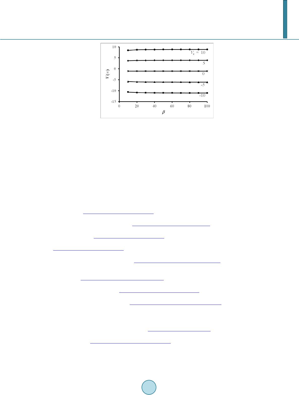

F. M. N. El-Fayez
129
Figure 4. Farfield normal velocity V(∞) vs. β , with different
values of Vs; m = 1. (Solid lines ≡ numerical, markers ≡ as-
ymptot ic).
5. Conclusion
The limiting behavior of the MHD flow due to a porous stretching sheet has been studied, as the magnetic field
grows indefinitely, taking into consideration the Hall current. Three-term uniformly-valid asymptotic expansions
have been derived using parameter straining. The velocity components show sinusoidal behavior that attenuates
exponentially, as we move away from the surface. (When the Hall current is neglected, the exponential decay
becomes monotonic.) Finite difference solutions have also been calculated. The two-term asymptotic and the
numerical solutions have shown excellent agreement both qualitatively and quantitatively.
References
[1] Crane, L.J. and Angew, Z. (1970) Flow Past a Stretching Plate. Zeitschrift für angewandte Mathematik und Physik
ZAMP, 21, 645. http://dx.doi.org/10.1007/BF01587695
[2] Gupta, P.S. and Gupta, A.S. (1977) Heat and Mass Transfer on a Stretching Sheet with Suction or Blowing. Canadian
Journal of Chemical Engineering, 55, 744. http://dx.doi.org/10.1002/cjce.5450550619
[3] Andersson, H.I. (1995) An Exact Solution of the Navier-Stokes Equations for Magnetohydrodynamic Flow. Acta
Mechanica, 113, 241. http://dx.doi.org/10.1007/BF01212646
[4] Andersson, H.I. (2002) Slip Flow Past a Stretching Surface. Acta Mechanica, 158, 121.
http://dx.doi.org/10.1007/BF01463174
[5] Wang, C.Y. (2009) Analysis of Viscous Flow Due to a Stretching Sheet with Surface Slip and Suction. Nonlinear
Analysis: Real World Applications, 10, 375. http://dx.doi.org/10.1016/j.nonrwa.2007.09.013
[6] Abel, M.S. and Nandeppanavar, M.M. (2009) Heat Transfer in MHD Viscoelastic Boundary Layer Flow over a
Stretching Sheet with Non-Uniform Heat Source/Sink. Communications in Nonlinear Science and Numerical Simula-
tion, 14, 2120. http://dx.doi.org/10.1016/j.cnsns.2008.06.004
[7] Kumar, H. (2011) Heat Transfer over a Stretching Porous Sheet Subjected to Power Law Heat Flux in Presence of Heat
Source. Thermal Science, 15, S187. http://dx.doi.org/10.2298/TSCI100331074K
[8] Vajravelu, K. a nd Rollins, D. (2004) Hydromagnetic Flow of a Second Grade Fluid over a Stretching Sheet. Applied
Mathematics and Computation, 148, 783. http://dx.doi.org/10.1016/S0096-3003(02)00942-6
[9] Nayfe h, A.H. (1973) Perturbation Methods. John Wiley, New York.
[10] Sutton, G.W. and Sherman, A. (1965) Engineering Magnetohydrodyna mics. McGraw-Hill, New York.
[11] Keller, H.B. (1969) Accurate Difference Methods for Linear Ordinary Differential Systems Subject to Linear Con-
straints. SIAM Journal on Numerical Analysis, 6, 8. http://dx.doi.org/10.1137/0706002
[12] Pantokratoras, A. (2009) A Common Error Made in Investigation of Boundary Layer Flows. Applied Mathematical
Modelling, 33, 413. http://dx.doi.org/10.1016/j.apm.2007.11.009

F. M. N. El-Fayez
130
Appendix
Given below are the expressions and relations that define the different symbols appearing in Expansions (6). For
conciseness, let
2 21
cos ,s, ()in ,
a
Ee CSa
η
γηγηλγ
−−
==== +
(A1-4)
then
0s
vVλα=−
( A5)
1
f
,
1
g
and
1
v
are obtained from
222
11
(3 2α)f αγgλγγ++=−
(A6)
22
11
23αγf(αγ )g λαγ−++ =
(A7)
111 1
2vλ(γgαf)f/α=− ++
(A8)
c
and
c

satisfy
22 2
01 1
1
(3 22αγ)c αγc v(γgαf) λγ f+ +=++

(A9)
22 01 11
23 2αγc(αγ )cv (αgγf) λ αγf− ++=−−

(A10)
a
,
b
,
a

, and
b

satisfy
2 22
1
8623 /2αaαγbαγaλ(αγ)f−+=−

(A11)
2 22
1
682(3 )/2αγaαbαγbf γαλγα ++=−

(A12)
2 2211
28 6()/2αγaαaαγb gf α γλγα −+−=−+


(A13)
211
26 822αγbαγaαb f/λα g γ −++ =−


(A14)
ˆ
a
and
ˆ
b
satisfy
ˆ
ˆ
3αaγba−=
(A 15)
ˆ
ˆ3γaαbb+=
(A 16)
and finally
2
f
,
2
g
, and
2
v
are obtained from
2
f ca=−−
( A17)
2
g ca=−−

( A18)
2 22
ˆ
2vλ(γgαf )c/αa=− +−−
(A19)