 Journal of Power and Energy Engineering, 2014, 2, 704-711 Published Online April 2014 in SciRes. http://www.scirp.org/journal/jpee http://dx.doi.org/10.4236/jpee.2014.24094 How to cite this paper: Taiwo, A.S. and Oricha, J.Y. (2014) Modeling, Steady-State Analysis of a SEPIC dc-dc Converter Based on Switching Function and Harmonic Balance Technique. Journal of Power and Energy Engineering, 2, 704-711. http://dx.doi.org/10.4236/jpee.2014.24094 Modeling, Steady-State Analysis of a SEPIC dc-dc Converter Based on Switching Function and Harmonic Balance Technique Ajayi Samuel Taiwo, Joseph Yakubu Oricha Electrical and Computer Engineering Department, Ahmadu Bello University, Zaria, Nigeria Email: tz4dabest@gmail.com, okaitojyo@yahoo.co.uk Received November 2013 Abstract The paper presents modeling approach of a Single Ended Primary Inductance Converter (SEPIC) system. The complete model derivation of the SEPIC converter system has been presented in dif- ferent modes of operation. Steady state and small signal analysis was carried out on the converter dynamic equations using the method of Harmonic balance Technique. The steady state variables and their respective ripple quantities obtained were plotted against duty ratio D. The results ob- tained for a supply input voltage of to the converter at a duty ratio of , compares well with simulation results. Keywords SEPIC Conve rte r; Switching Function; Harmonic Balance Technique 1. Introduction Fourth order converter had made applications of power possible where the demand for such requires less input voltage and high output voltage. Zeta, Cuk and SEPIC converter are examples of these. These converters have the ability to either buck or boost the voltage applied to their inputs depending on their applications. Analysis of these converters using averaging technique and waveform approach for transient and steady state study is very tedious and takes much computational time because of two storage element inclusion to the circuit. Solar based systems find interesting application when used with these converters to furnish the load with power. The SEPIC converter system as an example could be integrated with rural lightening systems, solar water pumping, Tele- communication industries and electric vehicle charging systems due to it buck-boost abilities. Attempts have been made by authors in [1], to use SEPIC converter to determine the I-V characteristics of solar generators. The performance of a dc water pump set driven by a PV source through a boost converter is reported in [2]. Studies and analysis of a buck converter large signal average model around an operating point with constant power load was reported in [3]. In [4] a novel technique for selecting passive components for the power stage of fourth-order dc-dc converter for an optimize system frequency response is reported. The authors’ in [5] reported that dc-dc response characteristics and stability determination using state space averaging tech-  A. S. Taiwo, J. Y. Oricha nique are one key point for accurate performance of a dc-dc converter feeding a load with power. In [6] [7] a model and steady state analysis of their respective converters for different power source were set forth for dif- ferent operating condition of the load. In this paper a switching function based technique is presented. The derivatives are used to study the large signal and small signal dynamic behavior of the SEPIC converter on a large scale computer simulation in conti- nuous current mode (CCM). In view of these, the resulting non-linear equation obtained due to this switching function approach coupled with applying harmonic balance technique help to produce dynamic equations which predict the average and ripple quantities respectively. This paper is organized as follows: section II is the studied SEPIC converter it’s model derivations in CCM together with the harmonic balance technique, section III present Fourier series of the switching functions. Section IV is the simulation and steady state results. Section V is the conclusion. 2. Studied Converter Figure 1, Shows the circuit diagram of the SEPIC converter used for this paper, it consist of an input capacitor , which serves as a voltage bank to the input of the SEPIC converter. Two inductors and with each parasitic resistance and . Two capacitors and with each associate equivalent series parasitic resistance and . One active switch and a passive switch. For continuous conduction modes (CCM), there are two states of the switch within the switching period T. could be a Mosfet, power bipolar junction transistor (BJT), Insulated gate bipolar transistor (IGBT), or any high power switching device which is switched on by a pulse width modulation signal (PWM) generated from a control module. During the first switching in- terval is on for a period defined by , while is off. During the next interval is off and is on for a period within the interval . 2.1. Model Derivation Equation (1) Gives the equation that describes two modes of operations of the SEPIC converter. Note; , ; throughout this paper. ( ) ( ) ( ) ( ) 11112 11221 22112 212 121222 112121 2221 22 2 0221 2 1 LLLLCLC C LC LLLCL LC CL L C LLC CL C LL L pivirSirivv LpiS virSirSiiSv C pviSSi C pvSiiv rR vvSi i ϕ ϕβ ϕβ β βϕ −−×++×++ −−−+×−× −+ + ×− = = = = = + + +× (1) Current and voltages of the transistor and diode are; Figure 1. SEPIC converter. C 0 r L1 L 1 S1 I T r C1 C1 r L2 L 2 r C2 V C2 R L V 0 I d C2 V C1 I L2 - + + - I C2 I I L1 I C1 V + - + -S2  A. S. Taiwo, J. Y. Oricha ( ) ( ) [ ] 11 2 2 11221 21 22 1 2121 T LL TCLLC C d LL dLCC C i Sii vSriiv v iSii S v Sirvv ϕ ϕβ β + +−−+ = = = + − = − (2) 2.2. Harmonic Balance Technique The technique unlike transient analysis assumes that the circuit steady state consist of a sum of sinusoids that best describe the differential equations. The method will involve imposing on Equation s (1) and (2) values, with average values together with their respective a.c variations, (ripple quantities). From these analysis, the steady state response solution of the system can be obtained and their respective ripple quantities. These equations are used to predict the performance of the system at steady state. ( ) ( ) ( ) ( ) () ( ) ( ) ( ) ( ) 1 1011 2 2021 1 1011 2 2021 01 01 01 01 01 s s s s s s s s s j LL L j LL L j CC C j CCC j TT T j dd d j TT T j dd d j ii i iiRe ie iiRe ie vvReve vvRe ve iiReie iiReie vvRe ve vVRe ve SdRe d e vv θ θ θ θ θ θ θ θ θ = + = + = + = + = = + = + = + = + = + (3) whe r e ; , , , , , , , , , are the average (dc) values of supply voltage, ca- pacitor voltage , capacitor voltage , transistor voltage , diode voltage , inductor current , in- ductor current , transistor current, diode current and switching function . Moreso, , , , , , , , , are complex ripple harmonic peaks of capacitor voltage , capacitor voltage , inductor current , inductor current , transistor Current, diode current and switching function . Where I = 1, 2, 3···, whe r e angular switching frequency in radians/seconds and is time in seconds. For continuous conduc- tion mode (CCM), then the switching of the converter is conforms to this constraint . The Equatio ns (1) and (2) have been used for simulation of the model. Putting Equation (3) into Equations (1) and (2) and con- sequently applying harmonic balance technique separating the steady state and ripple quantities, the dynamic equations for the average quantities and their ripple quantities counterpart are derived. 3. Fourier Series of the Switching Function The switching function applied to Eq uations (1) and (2) presents some difficulties in getting analytical close- form solutions. In solving this problem Fourier analysis is applied to get rid of these discontinuities. The expres- sion for the average (dc) components of the switching function can be found for this analysis. The function so derived is used for the derivation of the dynamic equation for the average and ripple quantities using harmonic balance Technique. The technique adopted is an effective method for studying the steady state of the system; which encompasses average, ripple quantities and could be use to study the stability of the converter which is not reported in this paper.  A. S. Taiwo, J. Y. Oricha S = 1, for and S = 0, for The Fourier expression of the periodic sequence of the pulse can be represented by a trigonometric series represented of the form [8]. ( ) ( ) 01 sin n sn n ftaDn t ω ∞ = = ++∅ ∑ (4) whe r e: ( ) () ( ) ( ) ( ) 0 0 22 1 0 0 1 tan 2cos ? 2sin ? T n nn n n T ns T ns aftdt T D ab a b aftnt dt T bftnt dt T ω ω − = = + ∅= = = ∫ ∫ ∫ (5) is the period, represented as where denote the switching frequency. is the radian frequency define by For The average value and the ripple quantities can be quickly found as a decided advantage for the value of 1. For this case, ( ) 10 0 t DT ft DTt T ≤≤ =≤≤ (6) ( ) ( ) ( ) ( ) ( ) ( ) ( ) ( ) ( ) ( ) ( ) 0 0 10 1 0 1 1 0 1 22 11 10 2cos ? 1sin 2 2sin ? 11cos 2 1sin 21cos 2 DT s DT s a DTD T ad D aftnt dt T aD bftnt dt T bD dD D ω π π ω π π ππ π = − = = = = = = = − = + − ∫ ∫ (7) The results of Equation (7) put in to Equation (3) and substituted into Equation s (1) and (2), are used for steady state average quantity calculations and ripple quantity calculations which are as presented in the next sec- tion. 4. Simulation and Steady-State Results Discussions Table 1 shows the parameters of the SEPIC converter used for the computer simulation. Steady state computer 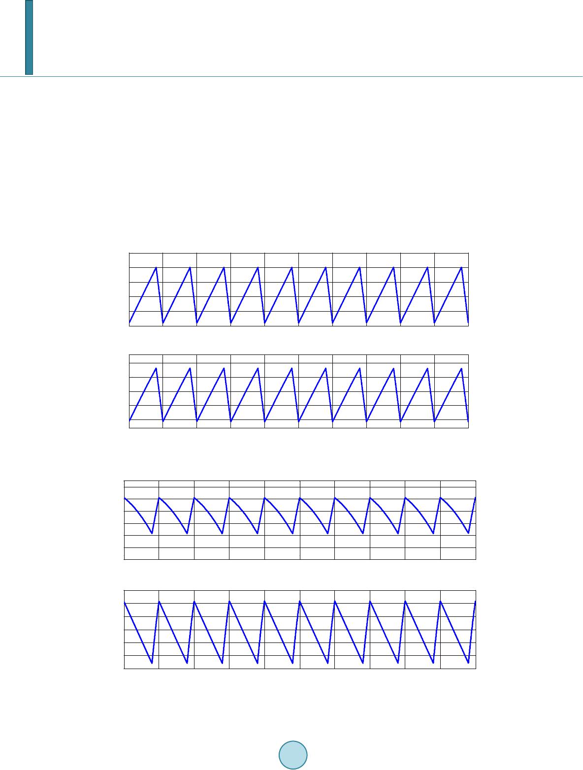 A. S. Taiwo, J. Y. Oricha simulation results for of the inductor currents, capacitor voltages show in Figure s 2 and 3. Voltages and currents impressed on the transistor and diode shown in Figures 4 and 5. The simulation and steady state results are ob- tained at duty ratio of 0.8. The steady state results plots against the duty ratio , is shown in Figure s 6 and 7. Also results for ripple quantities are shown in Figures 8 and 9. By comparing the simulation and calculated re- sults there is a good correlation between them Figures 2-5. Shows simulation results of the converter variables operating at duty cycle 0.8 the graph shows their simulation steady state results. Figure s 6-9 shows the result obtained after the application of harmonic balance technique to the converter model equations. A close observa- tion to the graph of Figure 6(f) shows that as the duty ratio varies between 0 and 0.9 the efficiency falls slightly. But as the duty ratio increases the efficiency falls significantly. In that note It can also be noted that av- erage value of the simulation graph of Figure 3(d) at a duty ratio of 0.8 are closed to that obtained from har- monic balance model at steady state at that particular point as shown in Figure 6. The graph of Figure 9 at a particular duty ratio give one the choice of selecting the voltage withstand capabilities of switching devices used. Figure 2. Simulation: state variables at steady state for . (a) ; (b) . Figure 3. Simulation: state variables at steady state for (c) ; (d) . 0.499 0.4991 0.4992 0.4993 0.4994 0.4995 0.4996 0.4997 0.4998 0.4999 0.5 85 90 95 100 105 110 (a) IL1 (A) 0.499 0.4991 0.4992 0.4993 0.4994 0.4995 0.4996 0.4997 0.4998 0.4999 0.5 15 20 25 30 35 (b) Time (s) IL2 (A) 0.4990.4991 0.4992 0.4993 0.4994 0.49950.4996 0.4997 0.4998 0.49990.5 52 54 56 58 60 62 64 (c) VC1 (V) 0.4990.4991 0.4992 0.4993 0.4994 0.49950.4996 0.4997 0.4998 0.49990.5 235 236 237 238 239 240 241 (d) Time (s) VC2 (V) 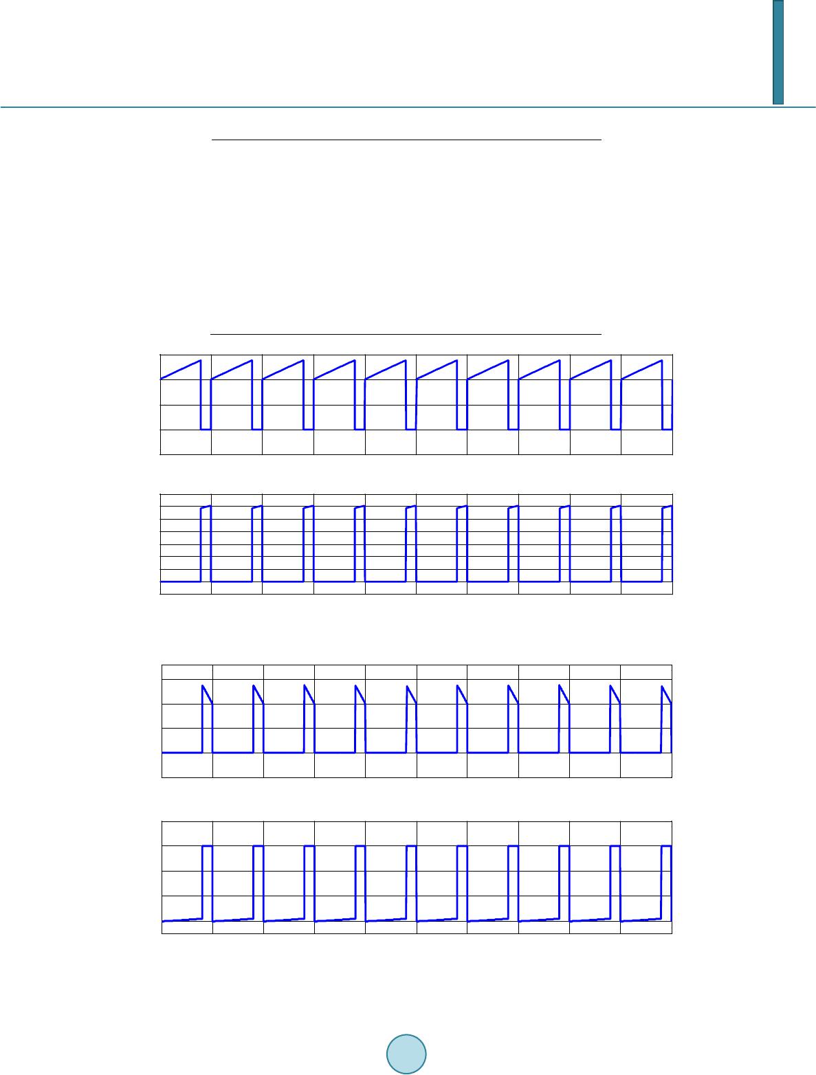 A. S. Taiwo, J. Y. Oricha Table 1. SEPIC converter parameters. voltage supply 60 V Inductance 250 µH uctanceInd 250 µH Capacitance 300 µF Capacitance 470 µF Rated load 10 Ω Duty ratio 0.8 switching Frequency 10 KHZ Figure 4 . Simulation: transistor current and voltage at steady state for . (e) ; (f) . Figure 5 . Simulation: diode current and voltage at steady state for . (g) ; (h) . 0.4990.4991 0.4992 0.4993 0.4994 0.49950.4996 0.4997 0.4998 0.4999 0.5 -50 0 50 100 150 (e) IT (A) 0.499 0.4991 0.4992 0.4993 0.4994 0.4995 0.4996 0.4997 0.4998 0.4999 0.5 -50 0 50 100 150 200 250 300 350 (f) Time (s) VT (V) 0.499 0.4991 0.4992 0.4993 0.4994 0.4995 0.4996 0.4997 0.4998 0.4999 0.5 -50 0 50 100 150 (g) Id (A) 0.499 0.4991 0.4992 0.4993 0.4994 0.4995 0.4996 0.4997 0.4998 0.4999 0.5 -300 -200 -100 0 100 (h) Time (s) Vd (V) 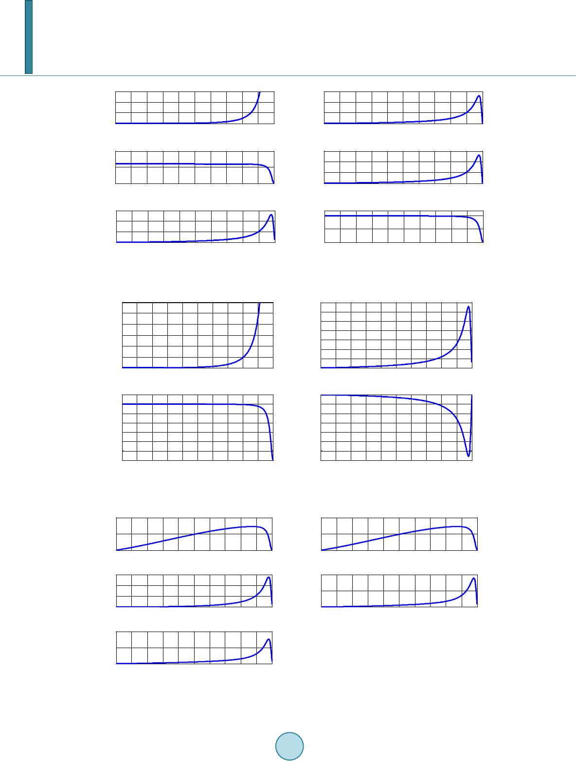 A. S. Taiwo, J. Y. Oricha Figure 6. Steady state average quantities (state variables), (a) 10L ; (b) ; (c) ; (d) ; (e) ; (f) . Figure 7. Steady state average quantities (devices current and voltage), (a) ; (b) ; (c) ; (d) . Figure 8 . Steady state average ripple quantities (state variables), (a) ; (b) ; (c) ; (d) ; (e) . 00.1 0.2 0.30.4 0.5 0.60.7 0.8 0.91 0 200 400 600 Input inductor current vs duty ratio i L10 (A) D (a) 00.1 0.2 0.30.4 0.5 0.60.7 0.8 0.91 0 50 100 150 Output inductor current vs duty ratio i L20 (A) D (b) 00.1 0.2 0.3 0.4 0.5 0.6 0.7 0.8 0.91 0 50 100 Intermediate Capacitor voltage vs duty ratio v C10 (V) D (c) 00.1 0.2 0.30.4 0.5 0.6 0.7 0.8 0.9 1 0 500 1000 1500 Output Capacitor voltage vs duty ratio v C20 (V) D (d) 00.1 0.2 0.30.4 0.5 0.60.7 0.8 0.91 0 500 1000 1500 Output voltage vs duty ratio v 00 (V) D (e) 00.1 0.2 0.30.4 0.5 0.60.7 0.8 0.91 0 50 100 Efficiency vs duty ratio η D (f) 00.1 0.2 0.3 0.4 0.5 0.6 0.7 0.8 0.9 1 0 100 200 300 400 500 600 Transistor T 1 Current vs duty ratio i T0 (A) D (a) 00.1 0.2 0.3 0.4 0.5 0.6 0.7 0.8 0.9 1 0 20 40 60 80 100 120 140 Diode d 1 Current vs duty ratio i d0 (A) D (c ) 00.1 0.2 0.3 0.4 0.5 0.6 0.7 0.8 0.9 1 0 10 20 30 40 50 60 70 Transistor T 1 Voltage vs duty ratio v T0 (V) D (b) 00.1 0.2 0.3 0.4 0.5 0.6 0.7 0.8 0.9 1 -1400 -1200 -1000 -800 -600 -400 -200 0 Diode d 1 voltage vs duty ratio v d0 (V) D (d) 00.1 0.2 0.30.4 0.5 0.60.7 0.8 0.91 0 5 10 Input inductor current ripple vs duty ratio i L11 (A) D (a) 00.1 0.2 0.30.4 0.5 0.60.7 0.8 0.91 0 5 10 Output inductor current ripple vs duty ratio i L21 (A) D (b) 00.1 0.2 0.30.4 0.5 0.60.7 0.8 0.91 0 5 10 15 Intermediate Capacitor ripple voltage vs duty ratio v C11 (V) D (c ) 00.1 0.2 0.30.4 0.5 0.60.7 0.8 0.91 0 5 10 Output Capacitor ripple voltage vs duty ratio v C21 (V) D (d) 00.1 0.2 0.30.4 0.5 0.60.7 0.8 0.91 0 5 10 Output ripple voltage vs duty ratio v 01 (V) D (e) 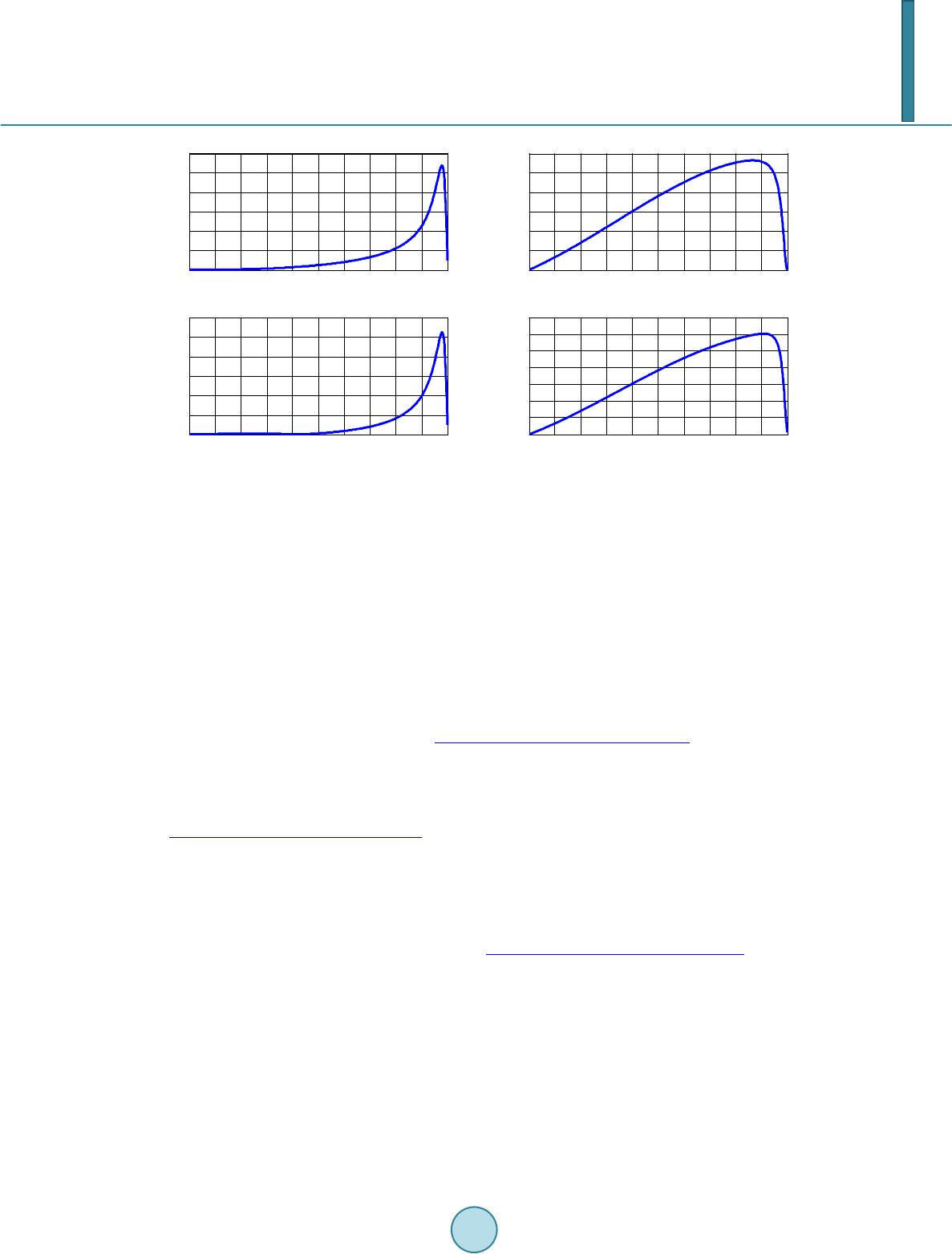 A. S. Taiwo, J. Y. Oricha Figure 9 . Steady state ripple quantities (devices current and voltage), (a) ; (b) ; (c) ; (d) . 5. Conclusion In this paper, the steady state and the dynamic behavior of the SEPIC converter are studied. Based on the graphs obtained, it can be seen that the results from the simulation and steady state results are in agreement. The har- monic balance technique simplifies the analysis for the non-linear equations of the state variables and devices. The steady state average and ripple quantity calculation was obtained by varying the duty ratio from 0 to 1. The advantage of the method is that switching stress withstand capability on the devices due to switching action can be predicted. References [1] Aranda, E.D., Galan, J. A.G., de Cardona, M.S. an d Marquez, J.M.A. (2009) Measuring the I-V Curve of PV Genera- tors. Industrial Electronic Magazine, 3, 4-14. http://dx.doi.org/10.1109/MIE.2009.933882 [2] Akbaba, M. and Akbaba, M.C. (2001) Dynamic Performance of a Photovoltaic-Boost Converter Powered dc Motor- Pump System. IEEE Electric Machines and Drive Conference, 356 -361. [3] Rivetta, C. an d Jayabalan, R. (2006) Analysis and Control of Buck dc-dc Converter Operating with Constant Power Load in Sea and Und ersea. IEEE Transaction on Industrial Applications, 42, 559-57 2. http://dx.doi.org/10.1109/TIA.2005.863903 [4] Nardo, A. D., Fermia, N., Nicolo, M., Petrone, G. and Soagnuolo, G. (2008) P o we r Stage Design of Fourth Order dc-dc Converter by Means of Principal Component Analysis. IEEE Transaction on Power Electronics, 23, 2867-2877. [5] Yang S., Goto K., Imamura, Y. and Shoyama, M. (2012 ) D ynamic Characteristics Model of Bi-Directional dc-dc Converter Using State Space Averaging Method. IEEE Telecommunications Energy Conference (INTELEC), 1-5. [6] Veerachar y, M. (20 12) Two-Loop Controlled Buck-SEPIC Converter for Input Source Power Managemen t. IEEE Transaction on Industrial Electronics, 59, 4075-4087. http://dx.doi.org/10.1109/TIE.2011.2174530 [7] Karimi -Davijani, H. and Ojo, O. (2011) Modeling and Steady-State Analysis of a Stan d-Alone Potovoltaic Three Phase Inverter Power System. IEEE Applied Electronics Conference and Exposition (APEC), 1259-12 66. [8] Edwin, K. (2006) Advance Engineering Mathematics. 9th Edition, Wiley International Edit io n . 00.1 0.2 0.3 0.4 0.5 0.6 0.7 0.8 0.9 1 0 50 100 150 200 250 300 Transistor T 1 Current ripple vs duty ratio i T1 (A) D (a) 00.1 0.2 0.3 0.4 0.5 0.6 0.7 0.8 0.9 1 0 20 40 60 80 100 120 Transistor T 1 Voltage ripple vs duty ratio v T1 (V) D (b) 00.1 0.2 0.3 0.4 0.5 0.6 0.7 0.8 0.9 1 0 50 100 150 200 250 300 Diode d 1 Current ripple vs duty ratio i d1 (A) D (c) 00.1 0.2 0.3 0.4 0.5 0.6 0.7 0.8 0.9 1 0 20 40 60 80 100 120 140 Diode d 1 voltage ripple vs duty ratio v d1 (V) D (d)
|