Applied Mathematics, 2011, 2, 496-503
doi:10.4236/am.2011.24064 Published Online April 2011 (http://www.SciRP.org/journal/am)
A Modified Discrete-Time Jacobi Waveform
Relaxation Iteration
Yong Liu1,2, Shulin Wu3
1Departme n t of Instrume n t Science and Engin ee ring, Southeast University, Nanjing, China
2Department of the Aeronautic Instruments and Electronic Engineering, The First Aeronautic Institute of Air Force,
Xinyang, China
3School of Science, Sichu an Universi t y of Science and Engineerin g, Zigong, China
Received November 7, 2010; revised March 11, 201 1; acce p ted M arch 14, 2011
Abstract
In this paper, we investigate an accelerated version of the discrete-time Jacobi waveform relaxation iteration
method. Based on the well known Chebyshev polynomial theory, we show that significant speed up can be
achieved by taking linear combinations of earlier iterates. The convergence and convergence speed of the
new iterative method are presented and it is shown that the convergence speed of the new iterative method is
sharper than that of the Jacobi method but blunter than that of the optimal SOR method. Moreover, at every
iteration the new iterative method needs almost equal co mputation work and memory storage with the Jacobi
method, and more importantly it can completely exploit the particular advantages of the Jacobi method in the
sense of parallelism. We validate our theoretical conclusions with numerical experiments.
Keywords: Discrete-Time Waveform Relaxation, Convergence, Parallel Computation, Chebyshev
Polynomial, Jacobi Iteration, Optimal SOR
1. Introduction
For very large scale initial value problems (IVPs), linear
or nonlinear, the waveform relaxation (WR) iteration,
also called dynamic iteration, is a very powerful method
and has received much interest from many researchers in
the past years, see [1-9] for more details about the history
of this method. The difference of the classical iteration
methods with the WR iteration method is that the WR
method iterates with functions in a func tional sp ace (con-
tinuous-time WR), and solve each iteration by some nu-
merical method (discrete-time WR), e.g. by the Runge-
Kutta methods. In the past years, both the continuous-
time WR iteration method and the discrete-time WR ite-
ration method have been investigated widely. For exam-
ple, one may refer to [1,3,9-13] for the the WR method
dis-cussed in continuous time level, and to [9,12, 14-17]
for the discrete-time WR method. There are so many ex-
cellent results in this field that we can not recount them
detaildly.
For the linear system of IVPs on arbitrarily long time
interval


0,T defined as
  


00
=,0,,
=,
ytyt fttT
yt y
 




H (1)
where 0
, :, ,
nnnn
fyy H


  , the Jacobi
WR iteration can be written as
  

111
0
d=,0=, =0,1,,
d
kkkk
yyyfy yk
t

 MN
(2)
where =

H
MN and M is a pointwise or block-
wise diagonal matrix. The discrete-time Jacobi WR ite-
ration can be obtained by applying some numerical me-
thod, such as BDF method, Runge-Kutta method, etc., to
discretize (2) for every iterative index k.
In Jacobi waveform relaxation, continuous-time or dis-
crete-time, system (2) is decoupled into, say d, loosely
coupled subsystems. If, on a parallel computer, these
subsystems are assigned to d different processors, and
they can be solved on


0,T simultaneously. This ob-
vious type of parallelism is present in all waveform re-
laxation methods, see, e.g., [1,2-4,9-12,15-19] and re-
ferences therein. However, in many cases, such as the
Gauss-Seidel, optimal SOR waveform relaxation methods,
exploiting this parallelism is only possible when appro-
ximations are exchanged between the different proce-
ssors as soon as they have been computed (see, e.g., [20]).
This leads to a large amount of communication during

Y. LIU ET AL. 497
each waveform relaxation sweep, which forms a severe
drawback. In Jacobi waveform relaxation, communica-
tion is only necessary once per sweep, and this method is
attractive for parallel implementation.
Therefore, we think that any improvement of the con-
vergence speed of the Jacobi WR iteration is important.
Based on this consideration, in this paper, we attempt to
get speed up by taking linear combinations of earlier Ja-
cobi iterates, and this leads to the following special ite-
rative scheme:
 





 
 
0
1
1
=0
for= 0,1,2,
=;
for=1,2, ,
d
=;
d
end
=;
end
k
mmm
km
m
m
k
xy
m
xt
x
txtft
t
yvx








MN (3)
where the parameters

=0
mm
v

are constant and satisfy
=0
=1.
m
m
v

 (4)
Since the discrete-time WR iteration is more favour-
able in practical applications, we will devote ourself to
getting the speed up of the discrete-time version of ite-
rative scheme (3). To solve the ODEs in (3), we first de-
compose the time interval


0,T into Ns sub-inter-
vals, say


1
,,=0,1,, 1
nn
ttnN s
, with equal leng-
th h. And then we solve (3) numerically by a linear
s
-step formula with coefficients

=0,1, ,
,
jj
j
s

, which
leads to the following iterative scheme written in
compact form as
 
 
 
 

 
0
0
0
1
=0 =0
1
=0
for= 0,1,2,
=,=0,1,,1;
=,=0,1,,
for=1,2, ,
=,=0,1,,1
for= 0,1,2,,
=;
end
end
=,=0,,;
end
k
jj
k
nn
m
jj
ss
mmm
jnjjnjnj nj
jj
km
nsm ns
m
k
yyj s
xyn Ns
m
xyjs
nN
xhxx f
yvxnN










 









MN
(5)
where the values

0,=0,1,,1
j
yj s are the
s
initial
values which are obtained by, for example, the backward
Euler method or some other one-step methods. We
denote the new iterative scheme (5) by Acc-Jacobi in the
remainder of this paper. We will show that the optimal
parameters

=0
mm
v

which are used to accelerate the
convergence of the original discrete-time Jacobi WR ite-
ration relate closely to the coefficients of the

-th Che-
byshev polynomial. Mor eover, the eff ects of the step size
h and the matrices , MN on the convergence speed of
the Acc-Jacobi method are also presented. We note that,
for the sake of economizing memory storage, formula (5)
can be performed in special wise which is independent of
the parameter

and nearly equals to that of the classi-
cal discrete-time Jacobi WR iteration.
The remainder of this paper is organized as follows. In
Section 2, we recall the definitions of the so-called

1
B
H
-
block matrix and M-matrix, and some related pr o p e r -t i e s.
In Section 3, the convergence speed of the discrete-time
WR iteration (5) is derived and some comparisons about
convergence speed between the Acc-Jacobi, the classical
Jac o bi a nd th e o p t imal S O R m ethods are given. In Section 4,
we presen t some nume rical re sults which v alidate ou r theo-
retical conclusions very well.
2. Some Basic Knowledge of Matrix
Throughout this paper, the partial orderings '


, '<

and the absolute value

in n
 and nn  are inter-
preted in componentwise. For a matrix nn



A
, let


qn

and


,=1, ,
i
nni q, be some positive inte-
gers satisfying =1 =
q
i
inn
. Then define the block-wise
vector and matrix spaces as follows (see also [11]):






1
1
==,,,,
=|=,
,is existfor=1 ,,.
Tn
nTT i
qqi
nn
qij
qq
nn
ij
ij ii
Vx
L
iq






 


xxxx
AAA
AA
(6)
Moreover, for any matrix nn G, let


11
=diag,,,=,
GnnGG
gg 
D
BDG
and 1 =,
GGG

J
DB (7)
provided that the quantities 0
ii
q, =1,2,,in.
Definition 1 ([21]). A real matrix

=ij nn a

A with
0
ij
a

for all ij

is an M-matrix if
A
is nonsi-
gular and 10
A.
Definition 2 ([11, 22]). q LH is an

1
B
H
-block
matrix, if its block comparison matrix
H
defined by

Y. LIU ET AL. 498
1
1,=1,,,
=,,,=1,,.
ii
ij
ij
iq
ijij q









H
HH (8)
is an
M
-matrix, here and hereafter  denotes the
standard Euclidean norm.
Clearly, any
M
-matrix

=ij aA with positive dia-
gonal elements is an

1
B
H
-block matrix.
For q LH, we use


=qq
ij 
HH to re-
present the block absolute value. The block absolute
value of a vector q Vx can be defined in a similar way,
i.e.,



1
=,, .
T
TT
q
xx x
Definition 3 ([21]). For nn

real matrices
H
, M
and N, =
H
MN is a regular splitting of matrix
H
, if M is nonsingular with 10 0and
MN.
Lemma 1 ([11, 22]). Let , , ,
qq
LVLMxy and

. Then
1)






 

];

 
LM LM
L
Mxyxyxy
2)













]
L
MLMMxMx;
3)







[]   MMxx;
4)
 


 MM
.
Lemma 2 ([11]). Let q LH be an

1
B
H
-block ma-
trix, then
1) isnonsingularH;
2) 1
1 



HH ;
3)

<1 
H
J,
where 1 =
H
HH
J
DB with

11
111
11
==,,
qq
diag 

 
H
HHH
JDBDH H and
=
H
H
B
HD .
Lemma 3 ([21]). Let =
H
MN
be a regular split-
ting of the matrix
H
. Then H is nonsingular with
10 H, if and only if

1<1


MN .
Lemma 4 ([21]). Let ,nn AB, satisfy 0AB .
Then
 
 
A
B.
Lemma 5 ([23]). Let nn 
H
, and can be splitted
as =


H
IB
, where >0, 0

B, then the follow-
ing results are equivalent:
1) 10
H;
2)

<

 B;
3) for =1,2,,in,

Re 0
i
 , where i

is the
eigenvalue of the matrix.
Lemma 6 ([21]). Let 10
H and
112 2
==
H
MN MN be two regular splittings of H.
Then

11
22 11
1> 0 

MNMN if 21 0NN ;

11
22 11
1>> >0 

MNMN if 21 0NN .
3. Convergence Analysis
As supposed in [11], we assume in this paper that the
matrix


nn
H and its splitting =

H
MN sa-
tisfy the following assumption.
Assumption (A). Assume that all the off diagonal ele-
ments of H are non-positive and H is a symmetric and

1
B
H
-block matrix; its splitting =
H
MN
satisfies for
some integer


1qqn

 that

11
=diag, , qq MHH
is a symmetric positive definite matrix and ,MN are
commutative matrices, i.e., =MNNM.
Under this assumption, we know that N is also a
symmetric matrix. Therefore, the eigenvalues of the pro-
duct MN are all real numbers, since for symmetric ma-
trices M and N, ,MN are commutative matrices if
and only if

=
T
MNMN , see, e.g., [21,23]. We next
make an assumption for the linear s-step formula as
follows.
Assumption (B). Assume that >0
s
s


, where
s

and
s

are the coefficients of the linear s-step formula.
Lemma 7. Let matrix H and its splitting =

H
MN
satisfy assumption (A). Then for any real number 0h,
h

IH is an
M
-matrix and


1<1h


IM N.
Proof. Since


11
=diag,, qq MHH is a symmetric
positive definite matrix with non-positive off diagonal
elements, by the conclusions 1, 3 of lemma 5 and the
results given in [11], we know that for any 0h it
holds
 
11
1
0and.hh


IMIMM
Clearly, the inequality

11
h IMM implies
11
0h




H
IH
D
D. Thus, by definition 3,
=hh h 
I
HIH
IH DB is a regular splitting of
matrix hIH and 11
hh



H
H
IH IH
D
BDB, since
=0
h
H
IH
BB, where the definition of the matrices
H
D
and
H
B
has been given in lemma 2.
Then it follows from lemma 4 and the conclusion 3 of
lemma 2 that



11
<1.
hh



HH
IH IH
DBDB (9)
Moreover, by definition 2 and the notations given in
lemma 2, it is clear that


=0
h IH
NB ,
=h h 
I
H
IM D and the matrix hIM is an
 1
B
H
-
block matrix, since

11
=diag,, qq MHH is a sym-

Y. LIU ET AL. 499
metric positive definite matrix.
Therefore, we have








11
1
1
=<1,
hh
hh
h












IH IH
IM NIMN
IM N
DB
(10)
where in the first, second and the last inequalities we
have used the conclusions 2, 4 of lemma 1, the con-
clusion 2 of lemma 2 and (9), respectively.
Finally, from (10) we know that


=
h
hIHIMN
is a regular splitting of matrix hIH which satisfies


1<1h


IH N. Hence, according to lemma 3, it
is easy to know that hIH is an M-matrix. □
Lemma 8 Let matrix H and its splitting =

H
MN
satisfy assumption (A). Then for any real number r, all the
eigenvalues of matrix

1
r IM N are real numbers.
Proof. In assumption (A), we have mentioned that the
matrices M and N are commutative. Therefore, by
the results in [21,23], we know that there exists a non-
singular matrix, say Q, such that


11
11
=diag, ,and
=diag,,,
MM
n
NN
n






QMQ
QNQ
where

=1
n
M
ii
 and

=1
n
N
ii
 are the real eigenvalues of
matrices M and N, respectively.
Thus, for any real nu mber r, it is obvious that the n
eigenvalues of the matrix

1
r IM N are
=1
n
N
iM
ii
r








,
which are real numbers. □
Now, we turn our attention to the convergence analysis
of the Acc-Jacobi method defined by (5). We denote the
convergent solution of the Acc-Jacobi method by ,
j
y
=0,1, ,jNs

 with

0
=
j
j
yy for =0,1, ,1js

.
We thus define the notations as Equation (11) shows.
Therefore, by careful routine calculations we can
equivalently rewritten the Acc-Jacobi iteration (5) as





1
11 1
==,
m
mk
mm

 
 
 

X
MNXMfrMN Yc
(12)
where




111
=0
=j
m
mj



 

cMNMfr
with

0
1= 

MN I . This implies the following relation bet-
ween

1k

Y and

k
Y as



11
=0 =0
=.
m
kk
mmm
mm
vv







 
YMNYc (13)
Hence, it follows from the convergence theory of Ja-
cobi iteration [21,23] that the vector

k
Y generated by
(13) converges to some value, say Y for example, if
and only if it holds that
 
11
=0 =0
=<1.
mm
mmss
mm
vv








 
MNN (14)
Therefore, we arrive at the following question: how to
select parameters

=0
mm
v

which minimize the argu-
ment



1
=0
m
mss
mv





N, and this leads to following
minimum problem
=1
01 =0
min ,
m
m
vv vm
vC








 (15a)
 





 














11
12
00 0
000
=0 =0
1
=0 =0=0
=,,, ,=,,, ,
=0,1,,,and =0,1,,
=,,,,0,,0
=,,,
TT
TT TTT T
mmmm kkkk
ssNss sNs
T
ss
TT T
jjj jjj
jj
ss s
TT
jjj jjNj
jj j
mk
hhyhhyhhy
hfhf hf

 
 
 





 
 
 
 

 




Xxxx Yyyy
rIH IHIH
f
11
01 01
01 01
,=, =,=0,1,,,
=,=
00
00 00
T
Tiii i i
ss
ss ss
ss
ss
ss
hhis 




























 

 


 


IMN N
N
NN
MN
NNN
N
NN N





  (11)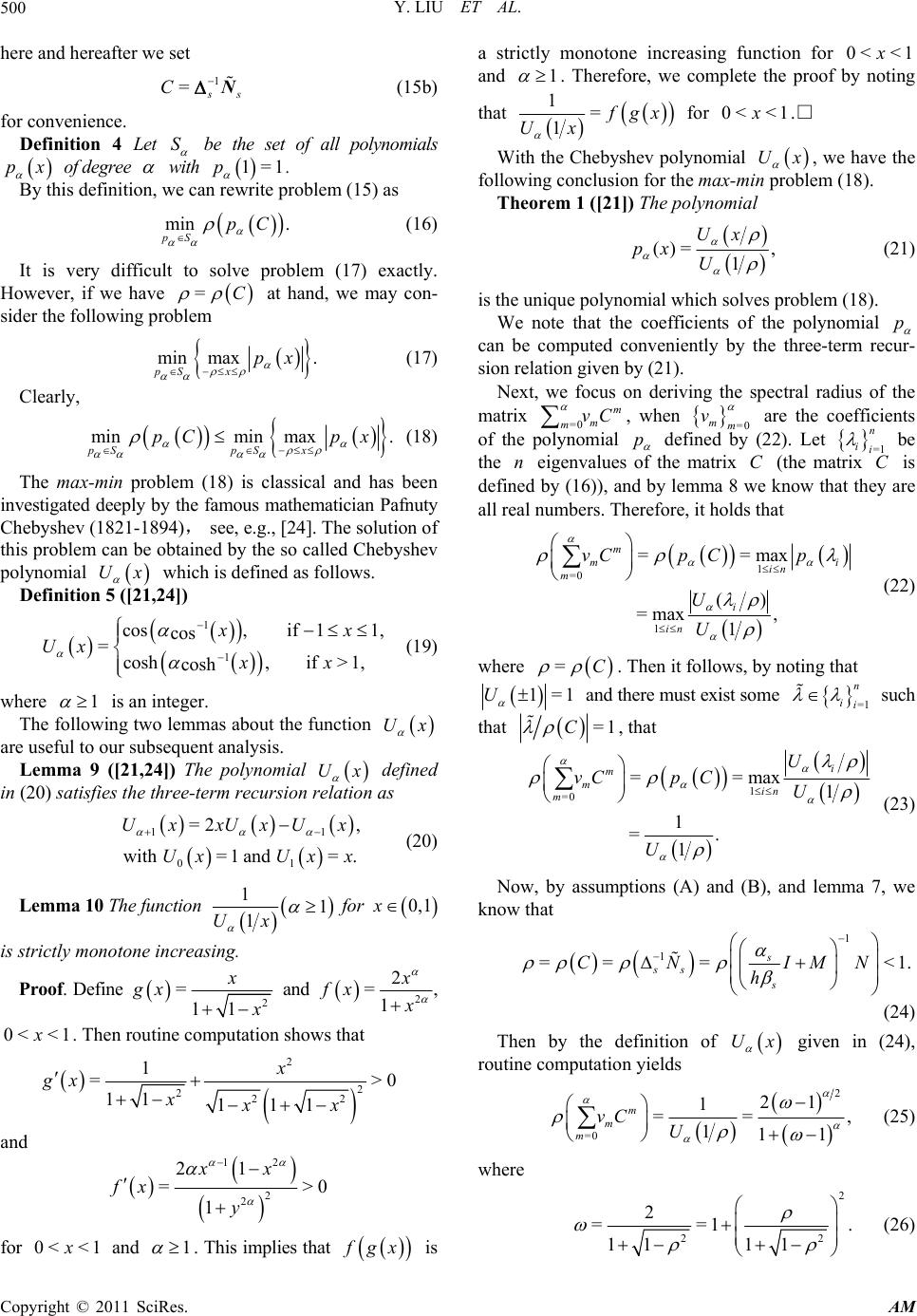

Y. LIU ET AL. 500
here and herea fte r we set
1
=
s
s
C N (15b)
for convenience.
Definition 4 Let S

be the set of all polynomials

px

of degree

with


1=1p

.
By this definition, we can rewrite problem (15) as
 
min .
pS pC



 (16)
It is very difficult to solve problem (17) exactly.
However, if we have


=C  at hand, we may con-
sider the following problem


min max.
pS xpx



 (17)
Clearly,




minmin max.
pSpS x
pC px


 

 
 (18)
The max-min problem (18) is classical and has been
investigated deeply by the famous mathematician Pafnuty
Chebyshev (182 1-1894)， see, e.g., [24]. The solution of
this problem can be obtained by the so called Cheb yshev
polynomial

Ux

which is defined as follows.
Definition 5 ( [21,24])
 



1
1
cos,if 11,
cos
=cosh,if >1,
cosh
xx
Ux xx





 




(19)
where 1

 is an integer.
The following two lemmas about the fun ction


Ux

are useful to our subsequent analysis.
Lemma 9 ([21,24]) The polynomial

Ux

defined
in (20) satisfies the three-term recursion relation as
 
 
11
01
=2 ,
with=1 and =.
Ux xUxUx
UxUx x
 
 (20)
Lemma 10 The function



11
1Ux

  for


0,1x
is strictly monotone increasing.
Proof. Define

2
=11
x
gx
x
 and

2
2
=1
x
fx
x


,
0< <1x. Then routine computation shows that


2
2
222
1
=>0
11 111
x
gx xxx

 
and




12
2
2
21
=>0
1
xx
fx y






for 0< <1x and 1

. This implies that

 
fgx is
a strictly monotone increasing function for 0<<1x
and 1

. Therefore, we complete the proof by noting
that
 

1=
1fgx Ux

for 0<<1x.□
With the Ch ebyshev polynomial


Ux

, we have the
following conclusion for the max-min probl em (18).
Theorem 1 ([21]) The polynomial


()= ,
1
Ux
px U





(21)
is the unique polynomial which solves problem (18).
We note that the coefficients of the polynomial p

can be computed conveniently by the three-term recur-
sion relation given by (21).
Next, we focus on deriving the spectral radius of the
matrix =0
m
m
mvC

, when

=0
mm
v

are the coefficients
of the polynomial p

defined by (22). Let

=1
n
ii
 be
the n eigenvalues of the matrix C (the matrix C is
defined by (16)), and by lemma 8 we know that they are
all real numbers. Therefore, it holds that
  

1
=0
1
==max
()
=max,
1
m
mi
in
m
i
in
vCp Cp
U
U














(22)
where


=C  . Then it follows, by noting that


1=1U

 and there must exist so me

=1
n
ii
 
 such
that


=1C 
, that
 



1
=0
==max
1
1
=.
1
i
m
min
m
U
vCp CU
U













 (23)
Now, by assumptions (A) and (B), and lemma 7, we
know that


1
1
== =<1.
s
ss s
CN IMN
h

 










(24)
Then by the definition of

Ux

given in (24),
routine computation yields



2
=0
21
1
== ,
111
m
m
m
vC U









 
 (25)
where
2
22
2
==1 .
11 11





 

(26)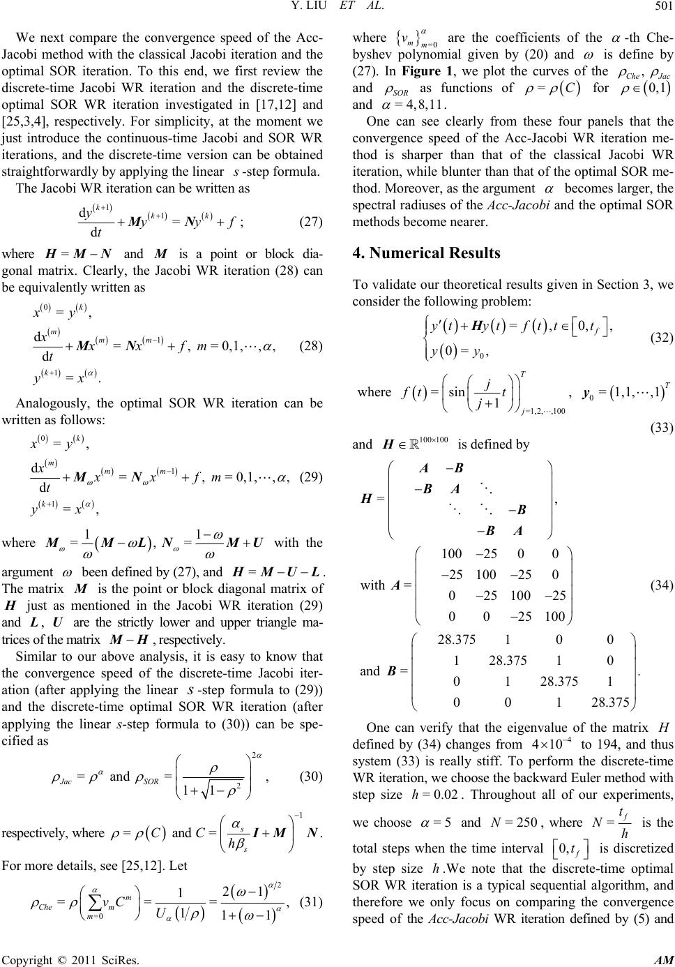

Y. LIU ET AL. 501
We next compare the convergence speed of the Acc-
Jacobi method with the classical Jacobi iteration and the
optimal SOR iteration. To this end, we first review the
discrete-time Jacobi WR iteration and the discrete-time
optimal SOR WR iteration investigated in [17,12] and
[25,3,4], respectively. For simplicity, at the moment we
just introduce the continuous-time Jacobi and SOR WR
iterations, and the discrete-time version can be obtained
straightforwardly by applying the linear
s
-step formula.
The Jacobi WR iteration can be written as
 
11
d=
d
kkk
yyyf
t

MN; (27)
where =
H
MN and M is a point or block dia-
gonal matrix. Clearly, the Jacobi WR iteration (28) can
be equivalently written as
 
  
 
0
1
1
=,
d=, =0,1,,,
d
=.
k
mmm
k
xy
xxxfm
t
yx




MN (28)
Analogously, the optimal SOR WR iteration can be
written as follows:
 
  
 
0
1
1
=,
d=, =0,1,,,
d
=,
k
mmm
k
xy
xxxfm
t
yx





MN (29)
where

11
=, =





 MMLN MU
with the
argument

been defined by (27), and =


H
MUL.
The matrix M is the point or block diagonal matrix of
H
just as mentioned in the Jacobi WR iteration (29)
and
L
, U are the strictly lower and upper triangle ma-
trices of the matrix MH, respectively.
Similar to our above analysis, it is easy to know that
the convergence speed of the discrete-time Jacobi iter-
ation (after applying the linear s-step formula to (29))
and the discrete-time optimal SOR WR iteration (after
applying the linear s-step formula to (30)) can be spe-
cified as 2
2
=and =,
11
Jac SOR



 





(30)
respectively, where

=C  and
1
=s
s
Ch







IM N.
For more details, see [25,12]. Let



2
=0
21
1
===,
111
m
Che m
m
vC U





 



 
 (31)
where

=0
mm
v

are the coefficients of the

-th Che-
byshev polynomial given by (20) and

is define by
(27). In Figure 1, we plot the curves of the ,
Che Jac


and SOR

as functions of

=C  for


0,1  
and =4,8,11

.
One can see clearly from these four panels that the
convergence speed of the Acc-Jacobi WR iteration me-
thod is sharper than that of the classical Jacobi WR
iteration, while blunter th an that of the optimal SOR me-
thod. Moreover, as the argument

becomes larger, the
spectral radiuses of the Acc-Jacobi and the optimal SOR
methods become nearer.
4. Numerical Results
To validate our theoretical results given in Section 3, we
consider the following problem:
 

0
=,0,,
0= ,
f
ytytfttt
yy






H (32)
where

=1,2, ,100
=sin 1
T
j
j
ftt
j








,

0=1,1, ,1
T
y
(33)
and 100 100


H
is defi ned by
=,
10025 00
25 100250
with =02510025
0025 100
28.375 100
128.37510
and =.
0128.375 1
001 28.375




























AB
BA
HB
BA
A
B
(34)
One can verify that the eigenvalue of the matrix
H
defined by (34) changes from 4 410

 to 194, and thus
system (33) is really stiff. To perform the discrete-time
WR iteration, we choose the backward Euler method with
step size =0.02h. Throughout all of our experiments,
we choose =5

and = 250N, where =
f
t
Nh is the
total steps when the time interval 0,
f
t


is discretized
by step size h.We note that the discrete-time optimal
SOR WR iteration is a typical sequential algorithm, and
therefore we only focus on comparing the convergence
speed of the Acc-Jacob i WR iteration defined by (5) and

Y. LIU ET AL. 502
Figure 1. The spectral radius of the three discrete-time WR iterative methods; from left to right: =4,8,11

.
Figure 2. Measured convergence speed of the Acc-Jacobi and discrete-time Jacobi WR methods.
Table 1. Coefficients

5
=0
mm
v for splitting =11 HM N

and =22 HM N.
coefficients

5
=0
mm
v
splitting 0
v 1 v 2 v 3 v 4 v 5 v
11
=HMN 0 0.041 468 677 620 310 0.561 375 694 613 35

0 1.519 907 016 993 04
22
=HM N 0 0.121 948 099 474 610 1.097 542 735 328 93

0 1.975 594 635 854 32
the Jacobi WR iteration. To make a fair comparison, the
discrete-time Jacobi WR iteration is performed as (29).
The measured error at iteration k for these two methods
is defined as:
 Jacobi:


1
Err= maxk
Jacn n
nN
kyy
 
  , where



=1
N
k
nn
y
 and

=1
N
nn
y
 are the k-th iterative solu-
tion and the convergent solution of the discrete-
time Jacobi WR method, respectively.
 Acc-Jacobi:


1
Err= maxk
Acc Jacnn
nN
kyy


, where


=1
N
k
nn
y and

=1
N
nn
y are the k-th iterative solu-
tion and the convergent solution of the Acc-Jacobi
method, respectively.
We choose two different splitting
112 2
==
H
MN MNwith

1=diag ,,,MAAA,


2=diag 100,100,,100Mand 11
=,NMH
22
=

NMH. And by computer it is easy to get
1
11
1
22
10.543 6,
1
and 0.666 7.
h
h






 






 




IM N
IM N
For the splitting 11 =
H
MN and 22 =

H
MN,
the coefficients

5
=0
mm
v are given in Table 1.
In Figure 2, we plot in the left and middle panels the
measured error decay of the two methods with splitting
11
=

H
MN and 22 =
H
MN, respectively, where
one can see clearly that the convergence speed of the
Acc-Jacobi method is much sharper than that of the
Jaocbi method. For these two splitting 11 =

H
MN

Y. LIU ET AL. 503
and 22 =
H
MN with 21 NN, theorem 1 predicts
that the Acc-Jacobi WR method with the former choice
shall converge faster than the case with the latter one.
This theoretical conclusion is clearly depicted in the right
panel of Figure 2.
5. Acknowledgments
This paper is supported by the the NSF of Sichuan Uni-
versity of Science and Engineering (2010XJKRL005,
2009JKRL011) and t he Si chu an Pro vi ncial Educat i on De-
partment Foundation of China (10ZB098). The authors
are grateful to the anonymous referees for the careful
rea-ding of a preliminary version of the manscript and
their valuable suggestions and comments, which really
improve the quality of this paper.
6. References
[1] C. Lubich and A. Ostermann, “Multi-grid Dynamic Itera-
tion for Pa rabolic Equations,” BIT Numerical Mathematics,
Vol. 27, No. 2, 1987, pp. 216-234.
doi:10.1007/BF01934186
[2] E. Lelarasmee, A. E. Ruehli and A. L. Sangiovanni-Vin-
centelli, “The Waveform Relaxation Methods for Time-
domain Analysis of Large Scale Integrated Circuits,”
IEEE Transactions on Computer-Aided Design of Inte-
grated Circuits and Systems, Vol. 1, No. 3, 1982, pp.
131-145. doi:10.1109/TCAD.1982.1270004
[3] U. Miekkala and O. Nevanlinna, “Convergence of Dy-
namic Iteration Methods for Initial Value Problems,”
SIAM Journal on Scientific and Statistical Computing,
Vol. 8, No. 4, 1987, pp. 459-482. doi:10.1137/0908046
[4] U. Miekkala and O. Nevanlinna, “Sets of Convergence
and Stability Regions,” BIT Numerical Mathematics, Vol.
27, No.4, 1987, pp. 554-584. doi:10.1007/BF01937277
[5] U. Miekkala, “Dynamic Iteration Methods Applied to
linear DAE Systems,” Journal of Computational and Ap-
plied Mathematics, Vol. 25, No. 2, 1989, pp. 133-151.
doi:10.1016/0377-0427(89)90044-7
[6] O. Nevanlinna, “Remarks on Picard-Lindelöf Iteration,
Part I,” BIT Numerical Mathematic, Vol. 29, No. 2, 1989,
pp. 328-346.
[7] O. Nevanlinna, “Remarks on Picard-Lindelöf Iteration,
Part II,” BIT Numerical Mathematic, Vol. 29, No. 3, 1989,
pp. 535-562. doi:10.1007/BF02219239
[8] O. Nevanlinna, “Linear Acceleration of Picard-Lindelöf
Iteration,” Numerische Mathematik, Vol. 57, No. 1, 1990,
pp. 147-156. doi:10.1007/BF01386404
[9] S. Vandewalle, “Parallel Multigrid Waveform Relaxation
for Parablic Problems,” B. G. Teubner, Stuttgart, 1993.
[10] J. Janssen and S. Vandewalle, “Multigrid Waveform
Relaxation of Spatial Finite Element Meshes: The Conti-
nuous-Time Case,” SIAM Journal on Numerical Analysis,
Vol. 33, No. 2, 1996, pp. 456-474. doi:10.1137/0733024
[11] J. Y. Pan and Z. Z. Bai, “On the Convergence of Wave-
form Relaxation Methods for Linear Initial Value Prob-
lems,” Journal of Computational Mathematics, Vol. 22,
No. 5, 2004, pp. 681-698.
[12] J. Sand and K. Burrage, “A Jacobi Waveform Relaxation
Method f or ODEs,” SIAM Journal on Scientific Com-
puting, Vol. 20, No. 2, 1998, pp. 534-552.
doi:10.1137/S1064827596306562
[13] J. Wang and Z. Z. Bai, “Convergence Analysis of Two-
stage Waveform Relaxation Method for the Initial Value
Problems,” Journal of Applied Mathematics and Compu-
ting, Vol. 172, No. 2, 2006, pp. 797-808.
doi:10.1016/j.amc.2004.11.031
[14] A. Bellen, Z. Jackiewicz and M. Zennaro, “Contractivity
of Waveform Relaxation Runge-Kutta Iterations and Re-
lated Limit Methods for Dissipative Systems in the Maxi-
mum Norm,” SIAM Journal on Numerical Analysis, Vol.
31, No. 2, 1994, pp. 499-523. doi:10.1137/0731027
[15] L. Galeone and R. Garrappa, “Convergence Analysis of
Time-Point Relaxation Iterates for Linear Systems of
Differential Equations,” Journal of Computational and
Applied Mathematics, Vol. 80, No. 2, 1997, pp. 183-195.
doi:10.1016/S0377-0427(97)00004-6
[16] R. Garrappa, “An Analysis of Convergence for Two-stage
Waveform Relaxation Methods,” Journal of Computa-
tional and Applied Mathematics, Vol. 169, No. 2, 2004,
pp. 377-392. doi:10.1016/j.cam.2003.12.031
[17] J. Janssen and S. Vandewalle, “Multigrid Waveform
Relaxation on Spatial Finite Element Meshes: The Dis-
crete-Time Case,” SIAM Journal on Scientific Computing,
Vol. 17, No. 1, 1996, pp. 133-155. doi:10.1137/0917011
[18] K. Burrage, Z. Jackiewicz and B. Welfert, “Block-Toe-
plitz Preconditioning for Static and Dynamic Linear Sys-
tems,” Linear Algebra and its Applications, Vol. 279, No.
1-3, 1998, pp. 51-74.
doi:10.1016/S0024-3795(98)00007-X
[19] J. M. Bahi, K. Rhofir and J. C. Miellou, “Parallel Solu-
tion of Linear DAEs by Multisplitting Waveform Relaxa-
tion Methods,” Linear Algebra and its Applications, Vol.
332-334, 2001, pp. 181-196.
doi:10.1016/S0024-3795(00)00199-3
[20] C. W. Gear, “Massive Parallelism Across Space in
ODEs,” Applied Numerical Mathematics, Vol. 11, No.
1-3, 1993, pp. 27-43. doi:10.1016/0168-9274(93)90038-S
[21] R. S. Varga, “Matrix Iterative Analysis,” Springer Verlag,
Berlin, New York, 2000. doi:10.1007/978-3-642-05156-2
[22] Z. Z. Bai, “Parallel Matrix Multisplitting Block Relaxa-
tion Iteration Methods,” Mathematica Numerica Sinica,
Vol. 17, No. 3, 1995, pp. 238-252.
[23] D. W. Young, “Iterative Solution of Large Linear Sys-
tems,” Academic Press, New York, 1971.
[24] J. C. Mason and D. C. Handscomb, “Chebyshev Poly-
nomials,” Chapman & Hall/CRC, Florida, 2003.
[25] J. Janssen and S. Vandewalle, “On SOR Waveform Re-
laxation Methods,” SIAM Journal on Numerical Analysis,
Vol. 34, No. 6, 1997, pp. 2456-2481.
doi:10.1137/S0036142995294292