Journal of Power and Energy Engineering, 2014, 2, 546-553
Published Online April 2014 in SciRes. http://www.scirp.org/journal/jpee
http://dx.doi.org/10.4236/jpee.2014.24074
How to cite this paper: Kamble, S. and Thorat, C. (2014) Voltage Sag Characterization in a Distribution Systems: A Case
Study. Journal of Power and Energy Engineering, 2, 546-553. http://dx.doi.org/10. 4236/jp ee .2014.24074
Voltage Sag Characterization in a
Distribution Systems: A Case Study
Suresh Kamble1, Chandrashekhar Thorat2
1Electrical Department, Government Polytechnic, Aurangabad, Maharashtra, India
2Principal Government Polytechnic, Aurangabad, Maharashtra, India
Received November 2013
Abstract
Voltage sags caused by the short-circuit faults in transmission and distribution lines have become
one of the most important power quality problems facing industrial customers and utilities. Vol-
tage sags are normally described by characteristics of both magnitude and duration, but phase-
angle jump should be taken into account in identifying sag phenomena and finding their solutions.
In this paper, voltage sags due to power system faults such as single phase-to-ground, phase-to-
phase, and two-phase-to-ground faults are characterized by using symmetrical component analy-
sis and their effect on the magnitude variation and phase-angle jumps for each phase are ex-
amined. A simple and practical method is proposed for voltage sag detection, by calculating RMS
voltage over a window of one-half cycle. The industrial distribution system at Bajaj hospital is
taken as a case study. Simulation studies have been performed by using MATLAB/SIMULINK and
the results are presented at various magnitudes, duration and phase-angle jumps.
Keywords
Power Quali ty ; Voltage S ag s ; Ch aracterizat ion
1. Introduction
According to IEEE standard 1159-1995, a voltage sag is defined as a decrease in rms voltage down to 90% to 10%
of nominal voltage for a time greater than 0.5 cycles of the power frequency but less than or equal to one minute
[1]. Voltage sags have always been present in power systems, but only during the past decades have customers
become more aware of the inconvenience caused by them [2].
Voltage sag may be caused by switching operations associated with a temporary disconnection of supply, the
flow of inrush currents associated with the starting of motor loads, or the flow of fault currents. These events
may emanate from the customers system or from the public network. Lighting strikes can cause momentary vol-
tage sags [3].
The interests in the voltage sags are increasing because they cause the detrimental effects on the several sensi-
tive equipments such as adjustable-speed drives, process-control equipments, programmable logic controllers,
robotics, computers and diagnostic systems, is sensitive to voltage sags. Malfunctioning or failure of this
equipment can cause by voltage sags leading to work or production stops with significant associated cost [4] [5].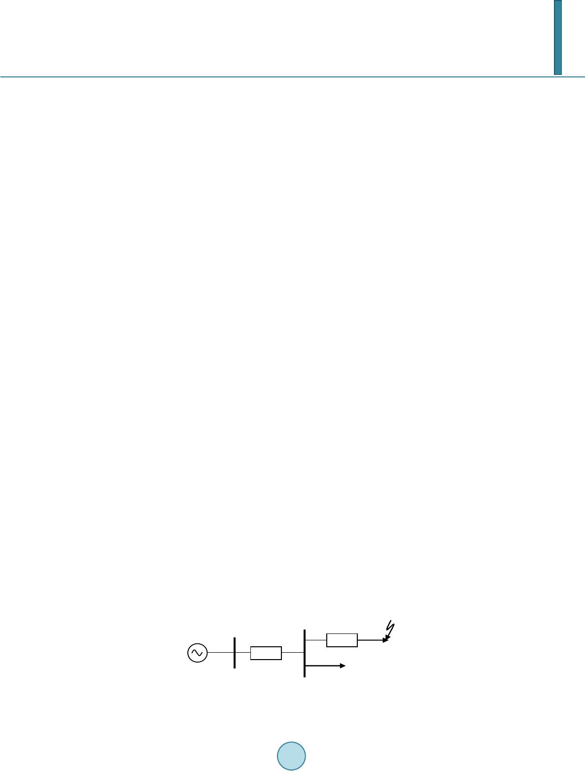

S. Kamble, C. Thorat
547
In the conventional method to assess these effects, voltage sags are characterized by its magnitude and dura-
tion. The magnitude is defined as the percentage of the remaining voltage during the sag and the duration is de-
fined as the time between the sag commencement and clearing [5]. However, balanced and unbalanced faults not
only cause a drop in the voltage magnitude but also cause change in the phase angle of the voltage. Therefore,
power–electronics converter that uses phase angle information for their firing instants may be affected by the
phase angle jump [6] [7]. In order to find any solutions for voltage sag problems due to faults, it is necessary to
identify characteristics of magnitude, duration and phase angle variations.
RMS (voltage or current) is a quantity commonly used in power systems as an easy way of accessing and de-
scribing power system phenomena. The rms value can be computed each time a new sample is obtained but
generally these values are updated each cycle or half cycle. If the rms values are updated every time a new sam-
ple is obtained, then the calculated rms series is called continuous. If the updating of rms is done with a certain
time interval, then the obtained rms is called discrete [7]. The analysis of different voltage sag characteristics of
different disturbances, a method using rms voltage to detect the voltage sag is proposed in this paper. The cor-
rectness of the method is proved by simulations.
In this paper, a comprehensive study is presented in order to show the proposed characterization of voltage
sags for the three types of faults, SLG, LL, and LLG. The algorithms for voltage sag detection and results by
using MATLAB/SIMULINK software.
2. Voltage Sag Characteristics
Voltage sag is defined as a decrease in rms voltage at the power frequency for durations of 0.5 cycles to 1
minute. This definition specifies two important parameters for voltage sag: the rms voltage and duration. The
standard also notes that to give a numerical value to a sag, the recommended usage is a sag 70%, which means
that the voltage is reduced down to 70% of the normal value, thus a remaining voltage of 30%. Sag magnitude is
defined as the remaining voltage during the event. The power systems faults not only cause a drop in voltage
magnitude but also cause change in the phase-angle of the voltage. The parameters used to characterize voltage
sag are magnitude, duration and phase angle jump.
2.1. Voltage Sag Magnitude
The magnitude of voltage sag can determine in a number of ways. The most common approach to obtain the sag
magnitude is to use rms voltage. There are other alternatives, e.g. fundamental rms voltage and peak voltage.
Hence the magnitude of the sag is considered as the residual voltage or remaining voltage during the event.
In the case of a three-phase system, voltage sag can also be characterized by the minimum RMS-voltage dur-
ing the sag. If the sag is symmetrical i.e. equally deep in all three phases, the lowest remaining voltage in any of
the phases can be used to characterize the sag. If the sag is unsymmetrical, i.e. the sag is not equally deep in all
three phases, the phase with the lowest remaining voltage is used to characterize the sag [8].
The magnitude of voltage sags at a certain point in the system depends mainly on the type and the resistance
of the fault, the distance to the fault and the system configuration. The calculation of the sag magnitude for a
fault somewhere within a radial distribution system requires the point of common coupling (pcc) between the
fault and the load to be found. Figure 1 shows the voltage divider model. Where Zs is the source impedance at
the pcc and ZF is the impedance between the pcc and the fault. In the voltage divider model, the load current be-
fore as well as during the fault is neglected. There is no voltage drop between the load and the pcc. The voltage
sag at the pcc equals the voltage at the equipment terminals, the voltage sag can be found from the Equation (1).
Figure 1. Voltage divider model.
pcc
V
sag
Z
s
Sensitive load
Fault
E
Z
F

S. Kamble, C. Thorat
548
F
sag F
Z
VE
Zs Z
=+
(1)
We will assume that the pre-event voltage is exactly 1 pu, thus E = 1. This result in the following expression
for the sag magnitude
F
sag F
Z
VZs Z =+
(2)
For fault closer to the pcc the sag becomes deeper (small
F
Z
). The sag becomes deeper for weaker supplies
(larger
S
Z
) [6].
2.2. Voltage Sag Duration
The duration of voltage sag is mainly determined by the fault–clearing time. The duration of a voltage sag is the
amount of time during which the voltage magnitude is below threshold is typically chosen as 90% of the nomin-
al voltage magnitude. For measurements in the three-phases systems the three rms voltages have to be consi-
dered to determine duration of the sag. The voltage sag starts when at least one of the rms voltages drops below
the sag-starting threshold. The sag ends when all three voltages have recovered above the sag-ending threshold
[9].
2.3. Phase Angle Jump
To obtain the phase-angle jump of a measured sag, the phase-angle of the voltage during the sag must be com-
pared with the phase-angle of the voltage before the sag. The phase-angle of the voltage can be obtained from
the voltage zero-crossing or from the phase of the fundamental component of the voltage. The complex funda-
mental voltage can be obtained by doing a Fourier transform on the signal. This enables the use of Fast-Fourier
Transform (FFT) algorithms. To explain an alternative method, consider the following voltage signal:
( )
( )( )
00
v tXcostYsint ωω = −
( )()
0
{
jt
v tReXjYe
ω
= +
(3)
with 0 the fundamental (angular) frequency. Two new signals are obtained from this signal, as follows:
( )( )
( )
0
22
d
vtv tcost ω = ×
(4 )
()( )
( )
0
22
q
vtv tsint ω = ×
(5)
which we can write as
( )
( )( )
00
22
d
v tXXcostYsint ωω =++
(6)
( )
( )( )
00
22
q
v tYYcostXsint ωω =−+ +
(7)
Averaging the two result signals over one-half cycle of the fundamental frequency gives the required funda-
mental voltage.
( )( )
dq
XjYvtjv t+= −
(8)
Knowing the values of X and Y, the sag magnitude can be calculated as
22
XY+
and the phase-angle
jump as
arctan Y
X
. This algorithm has been applied to detect the phase-angle jump. The effect of averaging
()
d
vt
and
()
q
vt
over one full cycle of the fundamental frequency is shown in Figure 3(c) for the phase-angle
jump. The effect of a larger window is that the transition is slower, but the overshoot in phase angle is less.
Which window length needs to be chosen depends on the application.
To understand the origin of phase-angle jump associated with voltage sags, the voltage divider model of Fig-
ure 1 can be used again, with the difference that Zs and
F
Z
are complex quantities which we will denote as
Zs
and
F
Z
. This gives for the voltage at the pcc.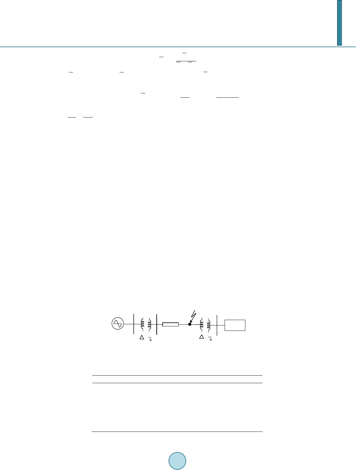

S. Kamble, C. Thorat
549
F
sag
F
Z
VZs Z =+
(9)
Let
ZsRs jXs= +
and
FsF
RX Zj = +
. The argument of
sag
V
, thus the phase-angle jump in the voltage, is
given by the following expression:
( )
argarctanarctan
sF
F
F sF
XX X
Vsag R RR φ
  +
∆==− 
 +
 
(10)
If
sF
sF
XX
RR
=
, expression (10) is zero and there is no phase-angle jump. The phase-angle jump will thus be
present if the X/R ratios of the source and the feeder are different [6] [10].
3. Simulation Study
Fault System Model
Figure 2 shows the single line diagram of the express feeder for Bajaj hospital under study. It is fed from 33/11
kv distribution substation of Maharashtra State Distribution Company Limited (MSEDCL), Railway station, In-
dustrial area, Aurangabad, India has been consider for voltage sag analysis. The system is modeled using the
simulink and Simpower System utilities of MATLAB. Table 1 shows system parameters used in the simulation.
The performance study of sample system is carried out for detection and characterization of voltage due to
power system faults. It is assumed that a fault has occurred at position F, on the primary side of distribution
transformer T2, and the fault lasted for 4 cycles from t = 0.045 to 0.125 seconds. The monitoring equipment is
installed at the pcc.
4. Simulation Results
4.1. Single Phase-to-Ground Fault
For simulation it is assumed that a single phase fault has appeared on phase A at position F. Phase voltages
waveform, rms voltages, and their phase angles are shown in Figure 3. The waveform shown in Figure 3(a)
shows an overvoltage at the end of the sag in faulted phase A. This overvoltage is almost certainly related to the
cause of the fault. The voltage of phase A drops nearly zero is up to 0.2 pu, while phases B and C voltages nor-
mally remains at pre-fault levels as shown in Figure 3(b). During the sag the voltage in the faulted phase Va is
suppressed with a large phase-angle jump (−48.92) degree, whereas the phase-angle jump in the other two non-
faulted phases is almost not affected. The duration of voltage sag in this case is 88 ms.
Figure 2. Single line diagram of distribution system for simu-
lation.
Table 1. Distribution system parameters.
Sr. No
Component
Details
1 Source 10 MVA, 33 kv, X/R = 10
2 Transformer T1 5 MVA, 33/11 kv, %Z = 7.15, X/R = 10, DYn11
3 Transformer T2 750 KVA, 11/0.433 kv, %Z = 5, X/R = 6, DYn11
4 Line 0.6748 + j0.372/km, 2 km
5 Load 208 KW and 130 KVAR
6 Frequency 50 Hz
L in e
Utility
F
pcc
Load
Y
Y
T1
T2

S. Kamble, C. Thorat
550
(a)
(b)
(c)
Figure 3. Single-phase-to-ground fault (a) voltage waveform; (b) rms voltage sag magnitude; (c) phase-angle jump.
4.2. Phase-to-Phase Fault
In addition to single phase-to-ground faults, the phase-to-phase faults also cause voltage sag. However, charac-
teristics for magnitude changes and phase-angle jump are not similar to those of SLG faults. Figure 4 shows the
00.02 0.040.06 0.08 0.1 0.120.14 0.160.18 0.2
-1.5
-1
-0.5
0
0.5
1
1.5
Voltage (pu)
Time (seconds)
Va
Vb
Vc
00.02 0.04 0.06 0.08 0.1 0.12 0.140.16 0.18 0.2
0
0 .1
0 .2
0 .3
0 .4
0 .5
0 .6
0 .7
0 .8
0 .9
1
1 .1
X: 0.04609
Y: 0.8992
Voltage Magnitude (pu)
Time (seconds)
X: 0.1341
Y: 0.9012
Va
Sag magnitude or Retained volatge
Duration
Threshold voltage V=90%
00.02 0.04 0.06 0.08 0.1 0.12 0.14 0.16 0.180 .2
-100
-90
-80
-70
-60
-50
-40
-30
-20
-10
0
Phase-angle jump (deg)
Time (seconds)
phase A
48.92

S. Kamble, C. Thorat
551
(a)
(b)
(c)
Figure 4. Phase-to-phase fault (a) Three-phase voltage waveform; (b) rms voltage sag mag-
nitude for phase A, B and C; (c) Phase-angle jumps for phase A, B and C.
00.02 0.04 0.06 0.08 0.1 0.12 0.14 0.16 0.18 0.2
-1
0
1
Phase-A voltage (pu)
00.02 0.04 0.06 0.08 0.1 0.12 0.14 0.16 0.18 0.2
-1.5
-1
-0.5
0
0.5
1
1.5
Phase-B voltage (pu)
00.02 0.04 0.06 0.08 0.1 0.12 0.14 0.16 0.18 0.2
-1
0
1
Phase-C voltage (pu)
Time (seconds)
Va
Vb
Vc
00.020.040.060.08 0.1 0.120.140.160.18 0.2
0
0.1
0.2
0.3
0.4
0.5
0.6
0.7
0.8
0.9
1
1.1
Voltage magnitude in pu
Time (seconds)
Va
Vb
Vc
V=90%
00.02 0.04 0.06 0.080.1 0.12 0.14 0.16 0.180.2
-100
-50
0
Phase-angle jump(deg)
Phase-A
00.02 0.04 0.06 0.080.1 0.12 0.14 0.16 0.180.2
-200
-100
0
100
200
Phase-angle jump(deg)
Phase-B
00.02 0.04 0.06 0.080.1 0.12 0.14 0.16 0.180.2
60
80
100
120
140
Phase-angle jump(deg)
Phase-C
Time (seconds)
phase a
phase b
phase c

S. Kamble, C. Thorat
552
voltage waveform, rms voltage and phase-angle jump characteristics for phase voltages due to phase-to-phase
fault between phases B and C. In Figure s 4(b) and (c), magnitudes and phase angles of phases B and C, with a
large voltage drop in the two phases Vb and Vc but phase voltage Va remains unchanged. The phase voltages
drop in magnitude Vb = 0.63 and Vc = 0.39 pu, The duration of voltage sag phases B = 80.72 ms, and C = 89.88
ms, and the phase-angle jumps are (+159) degree, and (+42) degree respectively.
4.3. Two Phase-to-Ground Fault
A voltage sags due to a two-phase-to-ground fault between phases B, C and ground. The voltage waveform, rms
voltages and phase-angle jump are recorded at the pcc as shown in Figure 5. This shows a significantly large
(a)
(b)
(c)
Figure 5. Two-Pha se-to-ground fault (a) Three-phase voltage waveform; (b) rms
voltage sag magnitude for phase A, B and C; (c) Phase-angle jumps for phase A, B
and C.
00.02 0.04 0.06 0.08 0.1 0.12 0.14 0.16 0.18 0.2
-1.5
-1
-0.5
0
0.5
1
1.5
Time (seconds)
Voltage (pu)
Va
Vb
Vc
00.020.04 0.06 0.080.1 0.12 0.14 0.160.180.2
0
0.2
0.4
0.6
0.8
1
Voltage magnitude in pu
Time (seconds)
Va
Vb
Vc
00.02 0.04 0.06 0.08 0.1 0.12 0.14 0.16 0.18 0.2
-100
-80
-60
-40
-20
0
Phase-angle jump (deg)
Phase-A
00.02 0.04 0.06 0.08 0.1 0.12 0.14 0.16 0.18 0.2
-200
-100
0
100
200
Phase-angle jump (deg)
Phase-B
00.02 0.04 0.06 0.08 0.1 0.12 0.14 0.16 0.18 0.2
20
40
60
80
100
Phase-angle jump (deg)
Phase-C
Time (seconds)

S. Kamble, C. Thorat
553
drop in rms voltage in the faulted phases B and C, but no change in phase A. The phase voltages drop in magni-
tude Vb = 0.2 and Vc = 0.2 pu, the duration of voltage sag phases B = 92.2 ms, and C = 88.9 ms, and the
phase-angle jumps are +160, and −41.7 degree respectively.
References
[1] (1995) IEEE Recommended Practice for Monitoring Electric Power Quality. IEEE Std. 1159-1995.
[2] Heine, P. and Lehtonen, M. (2003) Voltage Sag Distributions Caused by Power Systems Faults. IEEE Transactions on
Power Systems, 18, 1367-1373. http://dx.doi.org/10.1109/TPWRS.2003.818606
[3] Naidoo, R. and Pillay, P. (2007) A New Method of Voltage Sag and Swell Detection. IEEE Transactions on Power
Delivery, 22, 1056-1063. http://dx.doi.org/10.1109/TPWRD.2007.893185
[4] Juarez, E.E. and Hernandez, A. (2006) An Analytical Approach for Stochastic Assessment OG Balanced and Unba-
lanced Voltage Sags in Large Systems. IEEE Transactions on Power Delivery, 21, 1493-1500.
http://dx.doi.org/10.1109/TPWRD.2005.860266
[5] Wan, D.-J., Ahn, S.-J. and Chung, Y. (2003) A New Definition of Voltage Sag Duration Considering the Voltage To-
lerance Curve. IEEE Bologna Power Tech Conference, Bologna, 4, 23-26 June 2003.
[6] Bollen, M.H.J. (2000) Understanding Power Quality Problems: Voltage Sags and Interruptions. IEEE Press, New
York.
[7] Styvaktakis, E., Bollen, M.H.J. and Gu, I.Y.H. (2002) Automatic Classification on Power System Event Using RMS
Voltage Measurements. IEEE Power Engineering Society Summer Meeting, 2, 824-829.
[8] Ohrstrom, M. and Soder, L. (2003) A Comparison of Two Methods Used for Voltage Dip Characterization. IEEE
Power Tech Conference, Bologna, 4, 23-26 June 2003.
[9] Bollen, M.H.J. and Gu, I.Y.H. (2006) Signal Processing Of Power Quality Disturbances. IEEE Press.
http://dx.doi.org/10.1002/0471931314
[10] Zhang, L.D. and Bollen, M.H.J. (2000) Characteristic of Voltage Dips (Sags) in Power Systems. IEEE Transactions on
Power Delivery, 25, 827-832.