Journal of Power and Energy Engineering, 2014, 2, 483-488
Published Online April 2014 in SciRes. http://www.scirp.org/journal/jpee
http://dx.doi.org/10.4236/jpee.2014.24065
How to cite this paper: Miyauchi, H. and Misawa, T. (2014) Regression Analysis of Electric Power Market Price of JEPX.
Journal of Power and Energy Engineering, 2, 483-488. http://dx.doi.org/10.4236/jpee.2014.24065
Regression Analysis of Electric Power
Market Price of JEPX
Hajime Miyauchi1, Tetsuya Misawa2
1Department of Frontier Technology for Energy and Devices, Graduate School of Science and Technology,
Kumamoto University, Kumamoto, Japan
2Graduate School of Economics, Nagoya City University, Nagoya, Japan
Email: miyauchi@cs.kumamoto-u.ac.jp, misawa@econ.nagoya-cu.ac.jp
Received January 2014
Abstract
The deregulation of electric power industries is introd ucing around the world and electric power
markets are operated under the deregulation. Also in Japan, JEPX (Japan Electric Power Exchange)
operates a day-ahead market since April 2005. We have already analyzed the electric power mar-
ket prices in the several markets including JEPX by au t ore gre ssive models. We compose simple
regression equations, of which a dependent variable is the market price and explanatory variables
are the demand and the market price of 24 hours ago. In this paper, we analyze JEPX price data in
summer seasons from 2007 to 2013. In this period, the JEPX price is affected by many social phe-
nomena such as Lehman Shock and East Japan earthquake disasters. We compare the d ete rmin a-
tion coefficient and the coefficients of regression and investigate the change of coefficients over
the years.
Keywords
Market Price; JEPX; Autoregressive Model; Bidding Volume; Change over the Ye ars ; ADF Test
1. Introduction
The deregulation of electric power industries is progressing around the world. Many electric power markets are
also operated under the deregulated cir cumstance s. It is important to analyze the price in the electric power
markets. To analyze market prices, there are many analyzing tools. Nonlinear analysis, for examples, fuzzy
analysis and artificial neural networks, are sometimes very effective especially to forecast the future price.
However, the relation between input and output variables is not clear. On the other hand, linear analysis is es-
sential because the relation between input and output variables is clear. Therefore, we focus on the regression
model.
The electric power price in the deregulated California market has analyzed by the regression model [1]. We
also have been analyzing electric power prices by the regression equations in markets such as California, New
Engla nd , and so on [2] [3]. In order to analyze the prices in electric power markets, we compose a simple re-
gression equation of which a dependent variable is the market price and explanatory variables are the demand
and the market price of 24 hours ago.
Also in Japan, deregulation is progressing. The partial deregulation for the generation sector starts in 1995
H. Miyauchi, T. Misawa
484
and for the retail sector starts in 2000. Since April 2005, JEPX (Japan Electric Power Exchange) [4] opens a
day-ahead market when the deregulation in retail sector is expanded to the customers over 50 kW.
JEPX operates a day-ahead market for 9 years since then. We have analyzed the prices of JEPX by autore-
gressive model [5]. Though the variables used analyzing other markets are the market price, “System Price” is
analyzed for JEPX because the real market price of JEPX is not open. The system price is a virtual price as-
sumed that the market is unified excluding the different of frequency and congestion in transmission lines.
Moreover, as the every 30 minutes demand is not open in Japan, buying bid data of JEPX is used instead of de-
mand data. That is, the dependent variable of the regression equation is the system price and explanatory va-
riables are the buying bid and the system price of 24 hours ago.
In the analyzing period, JEPX system price is affected by many social phenomena such as Lehman Shock in
2008 and East Japan earthquake disasters in 2011. In this paper, we do not intend to analyze the effect of such
phenomena on the system price. However, autoregressive models of every year are compared and the change of
the price structure is investigated over the years.
2. Analyzed Data
2.1. JEPX Data
JEPX operates the day-ahead market since Apr 2005. Japanese power system is divided to the East Japan system
and the West-Central Japan system due to the difference of frequencies. Only 1200 MW can be transferred be-
tween two different frequency systems by 3 frequency converter sites. Moreover, transmission capacities of the
inter-ties between areas in each syst e m are also small. Then, a market sprit may often occur. JEPX does not
open a real price trading in the market. It opens only “System Price”, which is a virtual price assumed that the
market is unified in the whole country, excluding the difference of frequencies and congestions in transmission
lines. JEPX opens the system price of only two months ago and deletes the data from its open web site at the be-
ginning of the next month. The system price data is every 30 minute data according to the trading conditions of
electricity in Japan.
Demand data is employed in our former analysis for California and so on. However, every 30 minute demand
data is not released in Japan. Therefore, we use the buying bid data of JEPX instead of demand data. We have
already shown the effectiveness of the results using the buying bid data as an explanatory variable instead of
demand data [5].
Though we could obtain the system price data of JEPX from the beginning of its operation in 2005, we can
obtain the bid data of JEPX only from 2007. Therefore, we analyze the price data from 2007 to 2013. In this pa-
per, we analyze data only in summer season, that is, four months from June to September, as the summer is the
peak period of demand in Japan.
2.2. Scattering Diagram
Scattering diagrams between the system price and the buying bid of several years are shown in this chapter.
Figure 1 shows the scattering diagram of the summer in 2007. Though the scale of buying bid is very small,
the system price goes up to 60 JPY/kWh. Fig ures 2 and 3 show the scattering diagrams of the summer in 2009
and 2011. As the Lehman Shock occurred on 15 September 2008, year 2009 is the first year after the Lehman
Shock. The prices are affected severely by the decline of economy. On 11 March 2011, East Japan was attacked
by big earthquake and huge “tsunami” succeeding the earthquake. As many power plants in East Japan including
nuclear power plants were damaged, the electricity was not enough in summer 2011. The system price rises up
to about 40 JPY/kWh when the buying bid rises over 2 GW.
3. Regression Analysis
In this section, the regression equations [6] are derived according to the scattered diagrams shown in the pre-
vious section.
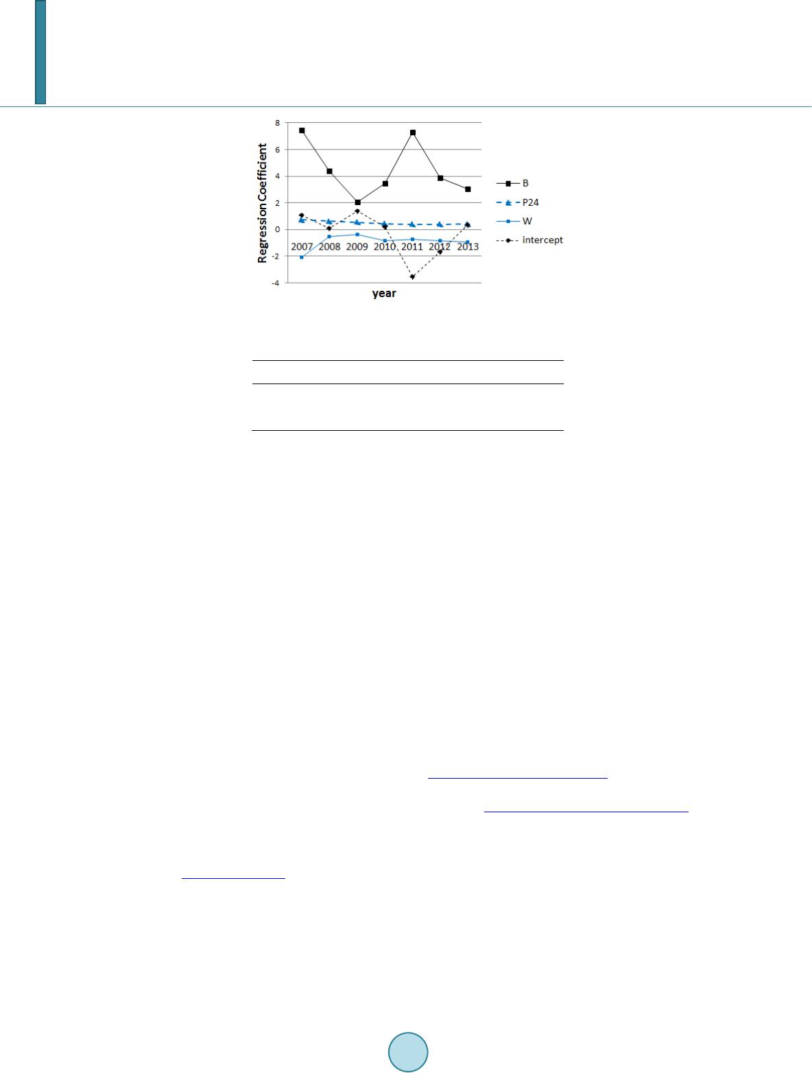
3.1. Regression Equations
We compose a simple regression equation. The dependent variable of the regression equations is the system
price P [JPY/kWh]. The explanatory variables are three variables, that is, the buying bid B [GW], the system
H. Miyauchi, T. Misawa
485
Figure 1. Scattering diagram between buying bid B [GW]
and system price P [JPY/kWh] in the summer 2007.
Figure 2. Scattering diagram between buying bid B [GW]
and system price P [JPY/kWh] in the summer 2009.
Figure 3. Scattering diagram between buying bid B [GW]
and system price P [JPY/kWh] in the summer 2011.
price at 24 hours ago P24 [JPY/kWh], and the dummy variable W which denotes Saturdays, Sundays and holi-
days as 1, and other weekdays as 0. We analyze 4 month data in summer (from June to September) of every year
between 2007 and 2013. The regression analysis is executed by the analyzing tool in Excel2010.
Regression equations are shown in Equations (1)-(7).
summer in 2007:
24
7.448 0.71562.0761.093PBP W=+ −+
(1)
(24.17) (92.25) (25.9 7) (10 . 28)
2
' 07430R=
H. Miyauchi, T. Misawa
486
summer in 2008:
24
4.368 0.62860.54370.07739PB PW=+ −+
(2)
(47.21) (85. 37) (12.78) (1.090)
2
' 0.8557R=
summer in 2009:
24
2.046 0.55720.34801.369PB PW=+ −+
(3)
(43.77) (65. 42) (19.68) (31.99)
2
' 07269R=
summer in 2010:
(4)
(37.06) (44.87) (12 .34) (1. 587 )
2' 0.5890R=
summer in 2011:
24
7.291 0.39550.74603.554
PB PW
=+ −−
(5)
(51.27) (40.66) (8.983) (20.89)
2
' 07115
R=
summer in 2012:
24
3.880 0.39780.84161.651
PB PW=+ −−
(6)
(48.21) (39.90) (12.07) (10.52)
2' 0.7070
R=
summer in 2013:
24
3.048 0.41140.95450.3633PB PW=+ −+
(7)
(48.30) (42. 17) (14.80) (2. 3 01)
2' 0.6629
R=
where, R2is the adjusted coefficient of determination. Values in parentheses under the regression coefficients
are “t-ratio, which present the individual significance of explanatory variables and interception. All explanatory
variables and interceptions except for several years (2008, 2010 and 2013 shown by the underline) are signifi-
cant because the 1% point of t-distribution is about 2.6. Next, F-test is executed to check whether the combina-
tion of explanatory variables is significant. The minimum F-value among these years is 2798 in 2010, which is
larger than the 1% point of F-distribution (about 3.8). Therefore, we can conclude that almost variables are sig-
nificant and the combination of these explanatory variables is also significant.
3.2. Change of Coefficient of Determination
First, the change of coefficient of determination over the year is investigated. Figure 4 shows the adjusted coef-
ficients of determination from 2007 to 2013.
The adjusted coefficients of determination are over 0.7 except for 2010 and 2013. As ones for 2010 and 2013 are
0.59 and 0.66 respectively, these values are not low comparatively. Then, we can think that the employed re-
gression equation is effective in spite of the simple model.
3.3. Change of Regression Coefficients
Next, the change of regression coefficients over the year is observed. Figure 5 shows the regression coefficients
from 2007 to 2013.
H. Miyauchi, T. Misawa
487
Figure 4 . Change of adjusted coefficient of determination.
The regression coefficients of the system price at 24 hours ago P24 are almost constant after 2010. The regres-
sion coefficients of Concerning P24 in 2007 and 2010 are 0.72 and 0.45, respectively. From 2011 to 2013, its
range is narrow between 0.395 and 0.411. It means that the system price does not refer the price of one day be-
fore gradually.
The regression coefficient of the dummy variable W becomes gradually large recently. The price deference
between weekdays and holidays is about 0.8 JPY/kWh recently.
On the other hand, the regression coefficient of the buying bid B changes violently over the year. In 2009 after
Lehman Shock, the regression coefficient declines to 2.04 JPY/kWh/GW. In 2011 after the big earthquake in
East Japan, it rises up to 7.29 JP Y /kW h/GW . At last, it falls down to 3.05 JPY/kWh/GW last year. It is thought
that the change is caused by the capacity of generators.
4. Augmented Dickey-Fuller Test
When the variables are not stationary and have trends, the regression analysis may show “spurious regression”,
in which the coefficient of determination becomes large value, even if the correlation between variables is low.
If the process has such trends, the regression analysis is meaningless.
Unit root test can be checked whether the process is stationary and whether the regression analysis does not
show spurious regression. Among several kinds of the unit root test, we employ Augmented Dickey-Fuller
(ADF) Test [7]. ADF test can check the serial correlation in the error term. A regression equation is assumed to
be shown as Equation (8).
11t tt
ya by
µ
=++
(8)
where
t
µ
is the error term. Equation (8) is modified to Equation (9).
11
( 1)
t tt
yab y
µ
∆=+−+
(9)
where
1t tt
yyy
∆= −
. If b1-1 is equal to 0, the unit root exists. If b1-1 is less than 0, the process is stationary.
ADF test for AR(2) is as follows:
1212 1
( 1)
tt tt
yab byby
µ
−−
∆=++ −−∆+
(10)
Similarly, If b1 + b2 1 is equal to 0, the unit root exists.
If t-value of ADF test is larger than the critical value, the null hypothesis is adopted that unit root exists in the
process. If t-value is smaller, the null hypothesis is dismissed and the process is thought to be stationary.
In this section, we only check the one month data in August 2009. The regression equation for August 2009 is
shown in equation (11).
August 2009:
24
2.257 0.58640.44391.018PBPW=+−+
(11)
(20.72) (35.74) (11.56) (11.46)
2
' 07304R=
The results of ADF test are listed in Table 1. As 5% critical vale is -2.863 and 10% critical value is -2.568,
the data of buying bid shows slightly weak stationary.
H. Miyauchi, T. Misawa
488
Figure 5 . Change of regression coefficients.
Table 1. Results of ADF test.
ADF t-ratio Lag Length
System Price -3.232 50
Buying Bid -2.698 48
However, we can conclude that the data in August 2009 does not have the unit root and the process is statio-
nary. The lag number is selected automatically based on AIC (Akaike Information Criterion). The obtained lag
number is 48 and 50. It means just one day (24 hours) because the data is every 30 minute time series data.
It is necessary to check if all data does not have the unit root. This is our future task.
5. Conclusions
In this paper, we analyze the JEPX system price by regression equations. Though a simple regression equation is
used, the regression coefficients are high. From the results, it is found that the system price becomes not to be
affected by the former price and the dummy variable represented holidays. On the contrary, the regression coef-
ficient for the buying bid changes violently. Finally, we check the process is stationary by ADF test.
We only execute simple analysis of JEPX price. We will correct the data and continue the analysis. Then, we
want to make clear the structure of the market price.
Acknowledgements
We thank N. Nishiyama, a graduate student of Kumamoto University, for his effort of the data analysis.
References
[1] Vucetic, S., Tomsovic, K. and Obradovic, Z. (2001) Discovering Price-Load Relationships in California’s Electric Mar-
ket. IEEE Transactions on Power Systems, 12, 280-286. http://dx.doi.org/10.1109/59.918299
[2] Miyauchi, H., Tatsuguchi, G. and Misawa, T. (2004) Regression Analysis of Electric Power Price in California Power
Excha nge. IEEJ Transactions on Power and Energy, 124, 199-206. http://dx.doi.org/10.1541/ieejpes.124.199
[3] Ito, T. , M iyauchi, H. and Misawa, T. (2007) Regression Analysis of Electric Power Market Price with New Meteoro-
logical Explanatory Variable. Proceedings of International Conference on Electrical Engineering 2007, Hong Kong,
8-12 July 2007.
[4] JEPX . http://www.jepx.org/
[5] Nish iyama, N., Miyauch i, H. and Misawa, T. (2009) Regression Analysis for System Price of JEPX. The Papers of
Joint Technical Meeting on Power Engineeringand Power Systems Engineering”. IEE Japan, Nagoya, 31 Jun-2
Aug 2009.
[6] Maddala, G.S. (19 92 ) Introduction to Econometrics. 2nd Edition, Prentice-Hall Inc.
[7] Na wata, K. (2009) Introduction to Econometric Analysis by EViews. As a kur a -Shoten.