Applied Mathematics, 2011, 2, 436-443
doi:10.4236/am.2011.24055 Published Online April 2011 (http://www.SciRP.org/journal/am)
Convergence Criterium of Numerical Chaotic Solutions
Based on Statistical Measures
Julio Cesar Bastos de Figueiredo1, Luis Diambra2, Coraci Pereira Malta3
1Escola Superior de Propaganda e Marketing (ESPM), São Paulo, Brasil
2Laboratorio de Biologia de Sistemas, Florencio Varela, Argentina
3Instituto de Física, Universidade de São Paulo, São Paulo, Brasil
Received January 25, 2011; revised February 22, 2011; accepted February 25, 2011
Abstract
Solutions of most nonlinear differential equations have to be obtained numerically. The time series obtained
by numerical integration will be a solution of the differential equation only if it is independent of the integra-
tion step h. A numerical solution is considered to have converged, when the difference between the time se-
ries for steps h and h/2 becomes smaller as h decreases. Unfortunately, this convergence criterium is unsuita-
ble in the case of a chaotic solution, due to the extreme sensitivity to initial conditions that is characteristic of
this kind of solution. We present here a criterium of convergence that involves the comparison of the attrac-
tors associated to the time series for integration time steps h and h/2. We show that the probability that the
chaotic attractors associated to these time series are the same increases monotonically as the integration step
h is decreased. The comparison of attractors is made using 1) the method of correlation integral, and 2) the
method of statistical distance of probability distributions.
Keywords: Chaotic Attractor, Statistical Measure, Numerical Integration
1. Introduction
When using as nonlinear models ordinary differential
equations (ODE’s) or delay differential equations (DDE’s),
it is necessary, in general, to resort to numerical simula-
tions for analyzing their dynamical behaviour. Numerical
solutions of differential equations are obtained by discre-
tizing them, and it should be recalled that solutions of the
continuous equation are always solutions of the discre-
tized equation but not vice-versa. The time series obtai-
ned by numerical integration will be a solution of the
continuous differential equation if it is independent of
the integration step h, indicating that convergence of the
numerical integration has been reached. Usually the cri-
terium of convergence of the numerical integration is
based on the direct comparison of the numerical time
series calculated using steps of integration h and h/2: the
difference between these time series should decrease as h
is decreased, and convergence is achieved when this dif-
ference is smaller than a given precision ε. It should be
remarked that the comparison has to be made after sta-
tionarity is reached, that is, the transient must be re-
moved before comparison is made.
Nonlinear systems can exhibit complex behaviour and,
in the case of chaotic solutions, the direct comparison of
the calculated time series, as the integration step is hal-
ved, is not appropriate for establishing numerical conver-
gence, due to their characteristic sensitivity to initial con-
ditions. In fact, it is very common the assertion that cha-
otic solutions do not converge (see, for instance, Teixeira
et al. (2007) [1], Yao and Hughes (2007) and (2008) [2,
3]. The sensitivity to initial conditions causes the blow
up of the difference between the time series calculated
using integration steps h and h/2, respectively, regardless
of it being initially extremely small (Teixeira et al. [1]
state that “for chaotic systems, numerical convergence
cannot be guaranteed forever”). Sauer (2002) [4] has
shown that numerical integration cannot produce appro-
ximate correct individual (or even average) chaotic tra-
jectories due to shadowing breakdown, even though it
may produce an approximately correct chaotic attractor.
So, in the case of chaotic solutions, as convergence crite-
rium of the numerical integration, we propose the com-
parison of the chaotic attractors associated with the ape-
riodic time series calculated using integration steps h and
h/2. The chaotic attractor is the object that is invariant,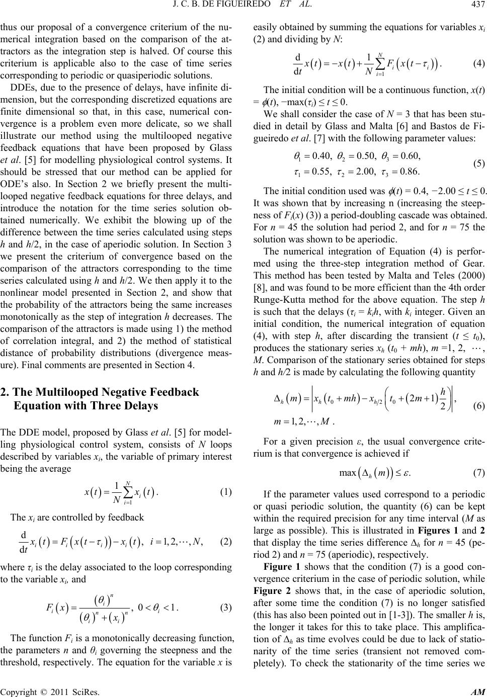

J. C. B. DE FIGUEIREDO ET AL. 437
thus our proposal of a convergence criterium of the nu-
merical integration based on the comparison of the at-
tractors as the integration step is halved. Of course this
criterium is applicable also to the case of time series
corresponding to periodic or quasiperiodic solutions.
DDEs, due to the presence of delays, have infinite di-
mension, but the corresponding discretized equations are
finite dimensional so that, in this case, numerical con-
vergence is a problem even more delicate, so we shall
illustrate our method using the multilooped negative
feedback equations that have been proposed by Glass
et al. [5] for modelling physiological control systems. It
should be stressed that our method can be applied for
ODE’s also. In Section 2 we briefly present the multi-
looped negative feedback equations for three delays, and
introduce the notation for the time series solution ob-
tained numerically. We exhibit the blowing up of the
difference between the time series calculated using steps
h and h/2, in the case of aperiodic solution. In Section 3
we present the criterium of convergence based on the
comparison of the attractors corresponding to the time
series calculated using h and h/2. We then apply it to the
nonlinear model presented in Section 2, and show that
the probability of the attractors being the same increases
monotonically as the step of integration h decreases. The
comparison of the attractors is made using 1) the method
of correlation integral, and 2) the method of statistical
distance of probability distributions (divergence meas-
ure). Final comments are presented in Section 4.
2. The Multilooped Negative Feedback
Equation with Three Delays
The DDE model, proposed by Glass et al. [5] for model-
ling physiological control system, consists of N loops
described by variables xi, the variable of primary interest
being the average
 
1
1.
N
i
i
x
txt
N
 (1)
The xi are controlled by feedback
   
d, 1,2,,,
dii ii
x
tFxt xtiN
t
   (2)
where τi is the delay associated to the loop corresponding
to the variable xi, and


 
, 01.
n
i
ii
nn
ii
Fx
x



 (3)
The function Fi is a monotonically decreasing function,
the parameters n and θi governing the steepness and the
threshold, respectively. The equation for the variable x is
easily obtained by summing the equations for variables xi
(2) and dividing by N:
 


1
d1 .
d
N
ii
i
xtxtF xt
tN


 
 (4)
The initial condition will be a continuous function, x(t)
=
 (t), −max(τi) ≤ t ≤ 0.
We shall consider the case of N = 3 that has been stu-
died in detail by Glass and Malta [6] and Bastos de Fi-
gueiredo et al. [7] with the following parameter values:
123
123
0.40, 0.50, 0.60,
0.55, 2.00, 0.86.




(5)
The initial condition used was
 (t) = 0.4, −2.00 ≤ t ≤ 0.
It was shown that by increasing n (increasing the steep-
ness of Fi(x) (3)) a period-doubling cascade was obtained.
For n = 45 the solution had period 2, and for n = 75 the
solution was shown to be aperiodic.
The numerical integration of Equation (4) is perfor-
med using the three-step integration method of Gear.
This method has been tested by Malta and Teles (2000)
[8], and was found to be more efficient than the 4th order
Runge-Kutta method for the above equation. The step h
is such that the delays (τi = kih, with ki integer. Given an
initial condition, the numerical integration of equation
(4), with step h, after discarding the transient (t ≤ t0),
produces the stationary series xh (t0 + mh), m =1, 2, ,
M. Comparison of the stationary series obtained for steps
h and h/2 is made by calculating the following quantity



020
21 ,
2
1, 2,,.
hh h
h
mxtmhxtm
mM

 



(6)
For a given precision ε, the usual convergence crite-
rium is that convergence is achieved if



max .
hm


 (7)
If the parameter values used correspond to a periodic
or quasi periodic solution, the quantity (6) can be kept
within the required precision for any time interval (M as
large as possible). This is illustrated in Figures 1 and 2
that display the time series difference ∆h for n = 45 (pe-
riod 2) and n = 75 (aperiodic), respectively.
Figure 1 shows that the condition (7) is a good con-
vergence criterium in the case of periodic solution, while
Figure 2 shows that, in the case of aperiodic solution,
after some time the condition (7) is no longer satisfied
(this has also been pointed out in [1-3]). The smaller h is,
the longer it takes for this to take place. This amplifica-
tion of ∆h as time evolves could be due to lack of statio-
narity of the time series (transient not removed com-
pletely). To check the stationarity of the time series we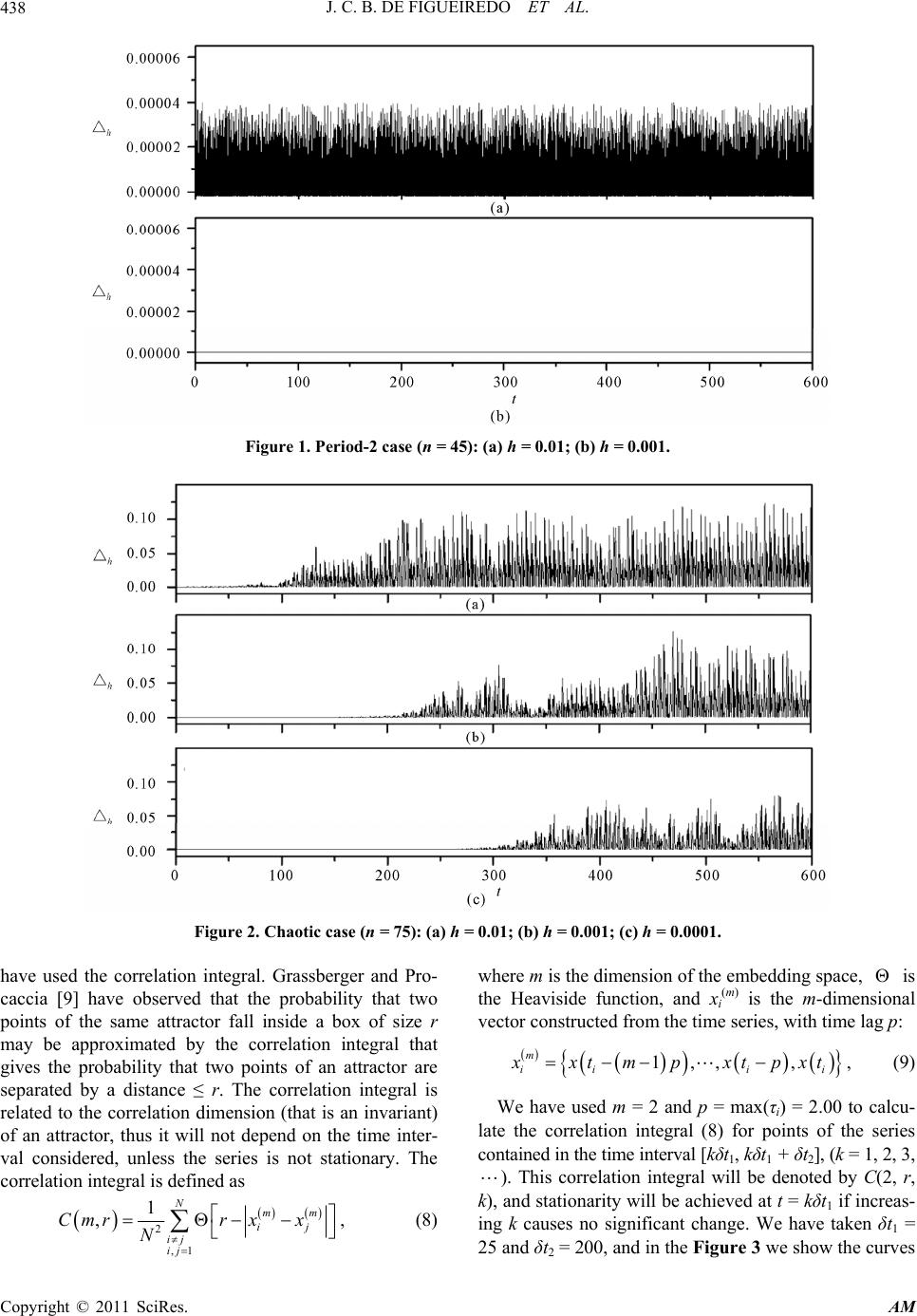

J. C. B. DE FIGUEIREDO ET AL. 438
Figure 1. Period-2 case (n = 45): (a) h = 0.01; (b) h = 0.001.
Figure 2. Chaotic case (n = 75): (a) h = 0.01; (b) h = 0.001; (c) h = 0.0001.
have used the correlation integral. Grassberger and Pro-
caccia [9] have observed that the probability that two
points of the same attractor fall inside a box of size r
may be approximated by the correlation integral that
gives the probability that two points of an attractor are
separated by a distance ≤ r. The correlation integral is
related to the correlation dimension (that is an invariant)
of an attractor, thus it will not depend on the time inter-
val considered, unless the series is not stationary. The
correlation integral is defined as

 
2
,1
1
,,
Nmm
ij
ij
ij
Cmrr xx
N



 (8)
where m is the dimension of the embedding space,

is
the Heaviside function, and xi
(m) is the m-dimensional
vector constructed from the time series, with time lag p:







1,,, ,
m
iii i
xxtmpxtpxt  (9)
We have used m = 2 and p = max(τi) = 2.00 to calcu-
late the correlation integral (8) for points of the series
contained in the time interval [kδt1, kδt1 + δt2], (k = 1, 2, 3,
). This correlation integral will be denoted by C(2, r,
k), and stationarity will be achieved at t = kδt1 if increas-
ing k causes no significant change. We have taken δt1 =
25 and δt2 = 200, and in the Figure 3 we show the curves

J. C. B. DE FIGUEIREDO ET AL. 439
Figure 3. Curves log C(2, r, k) × r, k = 1, 2, ···, 6 for the time
series with n = 75 calculated with step h = 0.0001 (same
time series used in the Figure 2(c)).
logC(2, r, k) × r for k = 1, 2, ···, 6. Stationarity is achie-
ved for k = 4 (t = 100) and this rules out the possibility of
the amplification of ∆h observed in Figure 2 being due to
nonstationarity effects. This indicates that the amplifica-
tion of ∆h observed in Figure 2 for the case n = 75, is a
consequence of the system dynamics.
3. Comparison of Attractors
Since the chaotic attractor is known to be invariant, we
propose that the criterium of convergence be based on
the comparison of the attractors associated with the time
series calculated using h and h/2 as integration step. We
shall present two procedures for comparing the attractors,
one based on the Kolmogorov-Smirnov test [10,11], and
another one based on the calculation of the attractors
divergence measure proposed by Diambra (2001) [12]. It
should be stressed that given any pair of time series,
these procedures can be used for comparing them.
3.1. Kolmogorov-Smirnov Test
The Kolmogorov-Smirnov test provides the probability
that two sets of measurements correspond to the same
distribution. Let

1
12
,,,
N
  and

2
12
,,,
N
  
be two sets of measurements of the same observable. The
corresponding cumulative distribution functions (not ex-
ceeding a given value η) are given by


1
1
2
2
1
1
1
2
1,
1.
N
Ni
i
N
Ni
i
N
N









(10)
The Kolmogorov-Smirnov statistics is defined as
 
12
,sup . NN
D
 




 
 (11)
Smirnov [11] has demonstrated that, given λ > 0, the
probability



,
122 12
112
Pr
21exp2 .
KS
j
j
QD
NN
jNN







 



 (12)
gives the significance of acceptance of the null hypothe-
sis that the two sets of data derive from the same distri-
bution.
Albano, Rapp and Passamante [13] proposed the use
of the correlation integral for calculating the Kolmogo-
rov-Smirnov statistics to be used for comparing the at-
tractors. The correlation for the 2-dimensional embed-
ding of the attractor corresponding to the time series xh
(t0 + mh), m = 1, 2, ···, M is


 
322
,,
2
3,1
1
2, ,
Mk
hihjh
ij
ij
Cr rxx
Mk





 (13)
where the integer k3 = τ3/h, and (2)
,
ih
x
is the ith vector of
the two-dimensional embedding of the attractor:








2
,0 03
3
,,
1, 2,,.
ih hh
x
xt ihxtikh
iMk
 

(14)
The Kolmogorov-Smirnov statistics related to the cor-
relation integral is given by
 
2min max
,2
max2,2, .
hh
CCh h
rrr
DCrCr

 (15)
We have calculated Ch(2, r) for r in the interval [0.01,
1.0] (N1 = N2 = 1000), using the time series resulting
from the numerical integration of the three delay equa-
tion with h = 0.01/2k, k = 0, 1, 2, ···, 9 (with parameter
values (5), t0 = 100). The results are displayed in Figure
4(a) and Figure 4(c) for n = 75, and n = 45, respectively.
In Figures 4(b) and 4(d) we display the corresponding
QKS, calculated using the statistics (15).
QKS, gives the probability that the attractors related to
the series calculated with time steps h and h/2 are the
same. Figure 4(b) shows that for the chaotic case (n =
75) this probability gets close to 100% for h ≤ 0.01/25
(probability is greater than 99.5%) while for the period-2
case (n = 45) (Figure 4(d)) this occurs for h = 0.01 (pro-
bability 100%). In the Figure 5 we display ∆h (6) for the
chaotic case with h = 0.01/28, and we can see the ampli-
fication of ∆h for t > 300.
3.2. Convergence Criterium Based on the
Statistical Distance
This method uses the divergence measure proposed by

J. C. B. DE FIGUEIREDO ET AL. 440
Figure 4. (a) and (c): correlation integral for the cases n = 75 and n = 45, respectively; (b) and (d): the corres-
ponding QKS calculated using the statistics (15) that is based on the correlation integral (h = 0.01/2k, k = 0,
1, ··· , 8).
Figure 5. ∆h, h = 0.01/28, that corresponds to the last point in the Figure 4(b) (chaotic case, n = 75).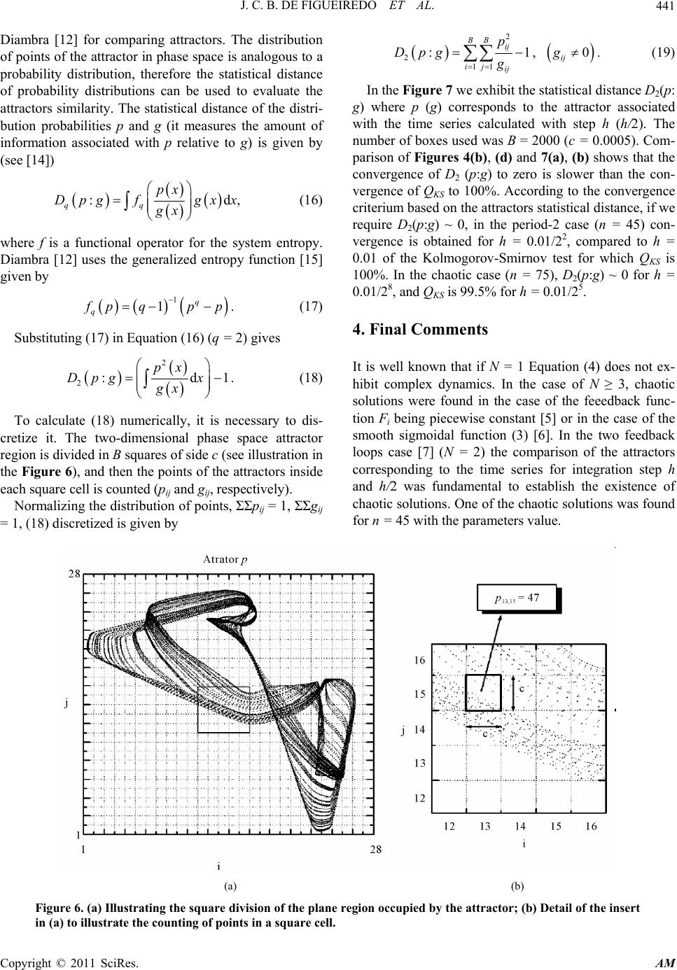

J. C. B. DE FIGUEIREDO ET AL. 441
Diambra [12] for comparing attractors. The distribution
of points of the attractor in phase space is analogous to a
probability distribution, therefore the statistical distance
of probability distributions can be used to evaluate the
attractors similarity. The statistical distance of the distri-
bution probabilities p and g (it measures the amount of
information associated with p relative to g) is given by
(see [14])
 
 
:d,
qq
px
Dpg fgxx
gx




 (16)
where f is a functional operator for the system entropy.
Diambra [12] uses the generalized entropy function [15]
given by
 

1
1.
q
q
f
pq pp

 (17)
Substituting (17) in Equation (16) (q = 2) gives
 

2
2:d1.
px
Dpg x
gx





 (18)
To calculate (18) numerically, it is necessary to dis-
cretize it. The two-dimensional phase space attractor
region is divided in B squares of side c (see illustration in
the Figure 6), and then the points of the attractors inside
each square cell is counted (pij and gij, respectively).
Normalizing the distribution of points, ΣΣpij = 1, ΣΣgij
= 1, (18) discretized is given by


2
2
11
:1, 0.
BB ij
ij
ij ij
p
Dpg g
g


 (19)
In the Figure 7 we exhibit the statistical distance D2(p:
g) where p (g) corresponds to the attractor associated
with the time series calculated with step h (h/2). The
number of boxes used was B = 2000 (c = 0.0005). Com-
parison of Figures 4(b), (d) and 7(a), (b) shows that the
convergence of D2 (p:g) to zero is slower than the con-
vergence of QKS to 100%. According to the convergence
criterium based on the attractors statistical distance, if we
require D2(p:g) ~ 0, in the period-2 case (n = 45) con-
vergence is obtained for h = 0.01/22, compared to h =
0.01 of the Kolmogorov-Smirnov test for which QKS is
100%. In the chaotic case (n = 75), D2(p:g) ~ 0 for h =
0.01/28, and QKS is 99.5% for h = 0.01/25.
4. Final Comments
It is well known that if N = 1 Equation (4) does not ex-
hibit complex dynamics. In the case of N ≥ 3, chaotic
solutions were found in the case of the feeedback func-
tion Fi being piecewise constant [5] or in the case of the
smooth sigmoidal function (3) [6]. In the two feedback
loops case [7] (N = 2) the comparison of the attractors
corresponding to the time series for integration step h
and h/2 was fundamental to establish the existence of
chaotic solutions. One of the chaotic solutions was found
for n = 45 with the parameters value.
(a) (b)
Figure 6. (a) Illustrating the square division of the plane region occupied by the attractor; (b) Detail of the insert
in (a) to illustrate the counting of points in a square cell.

J. C. B. DE FIGUEIREDO ET AL. 442
(a) (b)
Figure 7. Attractors statistical distance D2(p:g): (a) chaotic case (n = 75); (b) period-2 case (n = 45). The time se-
ries were calculated for h = 0.01/2k, k = 0, 1, ···, 8.
12
12
0.600, 0.510,
0.26, 2.00.




(20)
To confirm that this time series corresponded to a
chaotic solution, we constructed the bifurcation diagram,
displayed in the Figure 8, by varying n in the interval
[39,46] (computing 300 points in the Poincaré section for
each value of n).
The bifurcation diagram in Figure 8 shows the cha-
racteristic route of period-doubling bifurcation cascade
to chaos, indicating the existence of chaos in the
two-loops negative feedback system studied by Bastos de
Figueiredo et al. [7]. Our numerical investigation has
shown that the criterium of numerical convergence based
on the comparison of attractors corresponding to the time
series calculated using time steps h and h/2 (using either
(15) or (19)) works well for all types of solutions: peri-
odic, quasi-periodic or aperiodic. Figures 4 (Kolmogorov-
Smirnov test) and 7 (statistical distance) show that the
probability of the attractors being the same increases
(monotonically) as the step h is decreased.
In the period-2 case (n = 45) the Kolmogorov-Smir-
nov test (12) (using statistics (15)) indicates convergence
for h = 0.01 (see Figures 4(c) and 4(d)), and the test (19)
of attractors statistical distance gives the same result if
we require that D2(p:g) < 2.2 (see Figure 7(b)). If we
require that D2(p:g) < 1.0, it is necessary to use time step
h = 0.005. If we require D2(p:g) < 0.1, it is necessary to
use h = 0.0025. In the case of periodic or quasi-periodic
solutions it is possible to use (7) as convergence crite-
rium for the numerical integration. However, in the chao-
tic case (n = 75), due to the dynamical properties of this
type of solution, the difference (6) blows up as shown in
Figures 2 and 5. Nevertheless, the comparison of the
phase space chaotic attractors corresponding to the time
series calculated with time steps h and h/2 indicates that
the probability of the corresponding chaotic attractors
being the same increases monotonically as the time step
h decreases (see Figures 4(a) and 7(a)). For h = 0.001,
Figures 4(a) and 7(a) indicate that 87% < QKS < 93%,
and 2.0 < D2(p:g) < 3.0, respectively. Therefore the time
series calculated using h = 0.001 cannot be considered a
solution of the differential Equation (4) despite the fact
that (7), with ε = 0.000001, is satisfied for t < 100 (see
Figure 2(b)). It is necessary to use h ≤ 0.01/25 to obtain
a time series such that QKS ≥ 99.5% and D2(p:g) < 1.0
(see Figures 4(b) and 7(a)). Therefore, the fact that the
time series calculated by Teixeira et al. [1] satisfies con-
dition (7) during a certain time interval does not neces-
sarily mean that convergence has been achieved. It could
well be that their numerical integration has not conver-
ged as already pointed out by Yao and Hughes [2].
Our results indicate that D2(p:g) (Equation (19)) is
more sensitive than QKS (Equation (12)): the value of h
that gives probability ≥ 99.5% of the attractors being the
same corresponds to D2(p:g) < 1.0 (see Figures 4(b) and
7(a)). It is necessary to use h ≤ 0.01/28 to get D2(p:g) <
0.3.
Our method is very useful for detecting deviations
from a given reference time series that corresponds to a
behaviour that is desirable in a process being monitored
as in Stienstra et al. [16].

J. C. B. DE FIGUEIREDO ET AL. 443
Figure 8. Bifurcation diagram for two feedback loops with
parameters (20). The Poincaré section contains 300 points
for each value of n; We considered 100 values of n in the
interval [39,46].
5. Acknowledgements
The authors acknowledge financial support of CNPq
(Brazil). CPM also acknowledges support of FAPESP
(Brazil). L. D. is researcher of CONICET (Argentina).
6. References
[1] J. Teixeira, C. A. Reynolds and K. Judd, “Time Step Sen-
sitivity of Nonlinear Atmospheric Models: Numerical
Convergence, Truncation Error Growth, and Ensemble
Design,” Journal of the Atmospheric Sciences, Vol. 64,
No. 1, January 2007, pp. 175-189.
doi:10.1175/JAS3824.1
[2] L. S. Yao and D. Hughes, “Comment on ‘Time Step Sen-
sitivity of Nonlinear Atmospheric Models: Numerical
Convergence, Truncation Error Growth, and Ensemble
Design’,” Journal of the Atmospheric Sciences, Vol. 65,
No. 2, February 2007, pp. 681-682.
[3] L. S. Yao and D. Hughes, “Comment on ‘Computational
Periodicity as Observed in a Simple System, by E. N.
Lorenz’,” Tellus, Vol. 60, No. 4, August 2008, pp. 803-
805.
[4] T. D. Sauer, “Shadowing Breakdown and Large Errors in
Dynamical Simulations of Physical Systems,” Physical
Review E, Vol. 65, No. 3, March 2002, pp. 036220-1-5.
doi:10.1103/PhysRevE.65.036220
[5] L. Glass, A. Beuter and D. Larocque, “Time Delays, Os-
cillations and Chaos in Physiological Control Systems,”
Mathematical Biosciences, Vol. 90, No. 1-2, July-August
1988, pp. 111-125. doi:10.1016/0025-5564(88)90060-0
[6] L. Glass and C. P. Malta, “Chaos in Multi-Looped Nega-
tive Feedback Systems,” Journal of Theoretical Biology,
Vol. 145, No. 2, July 1990, pp. 217-223.
doi:10.1016/S0022-5193(05)80127-4
[7] J. C. B. de Figueiredo, L. Diambra, L. Glass and C. P.
Malta, “Chaos in Two-Loop Negative Feedback Sys-
tems,” Physical Review E, Vol. 65, No. 5, May 2002, pp.
051905-1-8. doi:10.1103/PhysRevE.65.051905
[8] C. P. Malta and M. L. S. Teles, “Nonlinear Delay Diffe-
rential Equations: Comparison of Integration Methods,”
International Journal of Applied Mathematics, Vol. 3, No
4, July 2000, pp. 379-395.
[9] P. Grassberger and I. Procaccia, “Measuring the Strange-
ness of Strange Attractors,” Physica D: Nonlinear Phe-
nomena, Vol. 9, No. 1-2, October 1983, pp. 189-208.
doi:10.1016/0167-2789(83)90298-1
[10] A. Kolmogorov, “Sulla Determinazione Empirica di um
Legge di Distribuizione,” Giornale Dell'Instituto Italiano
Degli Attuari, Vol. 4, 1933, pp. 83-91.
[11] N. Smirnov, “On the Estimation of Discrepancy between
Empirical Curves of Distribution for Two Independent
Samples,” Bulletin Mathématique de L´Université de
Moscow, Vol. 2, No. 2, 1939, pp. 3-11.
[12] L. Diambra, “Divergence Measure between Chaotic At-
tractors,” Physical Review E, Vol. 64, No. 3, September
2001, pp. 035202-1-5. doi:10.1103/PhysRevE.64.035202
[13] A. M. Albano, P. E. Rapp and A. Passamante, “Kolmo-
gorov-Smirnov Test Distinguishes Attractors with Similar
Dimensions,” Physical Review E, Vol. 52, No. 1, July
1995, pp. 196-205. doi:10.1103/PhysRevE.52.196
[14] I. Csiszár, “Statistical Decision Functions and Random
Processes,” Proceedings of 7th Prague Conference on
Information Theory, Prague, 1974, pp. 73-86.
[15] C. Tsallis, “Possible Generalization of Boltzmann-Gibbs
Statistics,” Journal of statistical physics, Vol. 52, No. 1-2,
July 1988, pp. 479-487. doi:10.1007/BF01016429
[16] G. J. Stienstra, J. Nijenhuis, T. Kroezen, C. M. van den
Bleek and J. R. van Ommen, “Monitoring Slurry-Loop
Reactors for Early Detection of Hydrodynamic Instabili-
ties,” Chemical Engineering and Processing, Vol. 44, No.
9, September 2005, pp. 959-968.
doi:10.1016/j.cep.2005.01.001