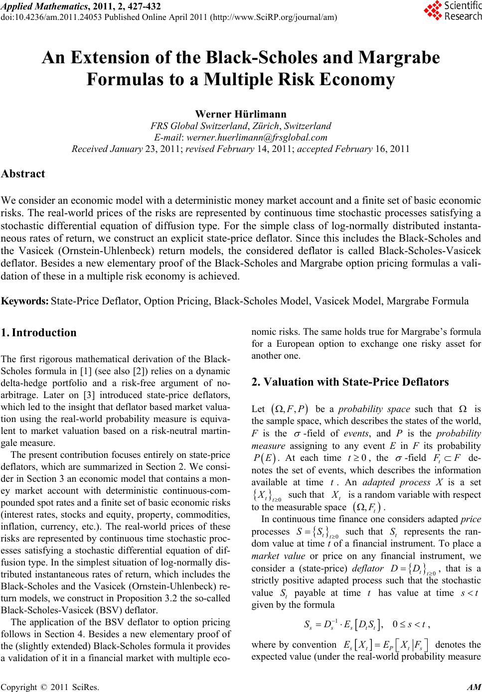Applied Mathematics, 2011, 2, 427-432
doi:10.4236/am.2011.24053 Published Online April 2011 (http://www.SciRP.org/journal/am)
An Extension of the Black-Scholes and Margrabe
Formulas to a Multiple Risk Economy
Werner Hürlimann
FRS Global Switzerland, Zürich, Switzerland
Received January 23, 2011; revised February 14, 2011; accepted Februar y 16, 2011
Abstract
We consider an economic model with a deterministic money market account and a finite set of basic economic
risks. The real-world prices of the risks are represented by continuous time stochastic processes satisfying a
stochastic differential equation of diffusion type. For the simple class of log-normally distributed instanta-
neous rates of return, we construct an explicit state-price deflator. Since this includes the Black-Scholes and
the Vasicek (Ornstein-Uhlenbeck) return models, the considered deflator is called Black-Scholes-Vasicek
deflator. Besides a new elementary proof of the Black-Scholes and Margrabe option pricing formulas a vali-
dation of these in a multiple risk economy is achieved.
Keywords: State-Price Deflator, Option Pricing, Black-Scholes Model, Vasicek Model, Margrabe Formula
1. Introduction
The first rigorous mathematical derivation of the Black-
Scholes formula in [1] (see also [2]) relies on a dynamic
delta-hedge portfolio and a risk-free argument of no-
arbitrage. Later on [3] introduced state-price deflators,
which led to the insight th at deflator based market valu a-
tion using the real-world probability measure is equiva-
lent to market valuation based on a risk-neutral martin-
gale measure.
The present contribution focuses entirely on state-price
deflators, which are summarized in Section 2. We consi-
der in Section 3 an economic model that contains a mon-
ey market account with deterministic continuous-com-
pounded spot rates and a finite set of basic economic risks
(interest rates, stocks and equity, property, commodities,
inflation, currency, etc.). The real-world prices of these
risks are represented by continuous time stochastic proc-
esses satisfying a stochastic differential equation of dif-
fusion type. In the simplest situation of log-normally dis-
tributed instantaneous rates of return, which includes the
Black-Scholes and the Vasicek (Ornstein-Uhlenbeck) re-
turn models, we construct in Proposition 3.2 the so-called
Black-Scholes-Vasicek (BSV) deflator.
The application of the BSV deflator to option pricing
follows in Section 4. Besides a new elementary proof of
the (slightly extended) Black-Scholes formula it provides
a validation of it in a financial market with multiple eco -
nomic risks. The same holds true for Margrabe’s formula
for a European option to exchange one risky asset for
another one.
2. Valuation with State-Price Deflators
Let


,,
F
P be a probability space such that

is
the sample space, which describes the states of the world,
F is the

-field of events, and P is the probability
measure assigning to any event E in F its probability


PE. At each time 0t, the

-field t
F
F de-
notes the set of events, which describes the information
available at time t. An adapted process X is a set


0
tt
X such that t
X
is a random variable with respect
to the measurable space


,t
F
.
In continuous time finance one considers adapted price
processes


0
tt
SS

 such that t S represents the ran-
dom value at time t of a financial instrument. To place a
market value or price on any financial instrument, we
consider a (state-price) deflator

0
tt
DD

, that is a
strictly positive adapted process such that the stochastic
value t S payable at time t has value at time
t
s

given by the f o rmula


1,0
ssstt
SDEDS st


,
where by convention


s
tPts
EXE XF denotes the
expected valu e (u nder the real-world p robability measure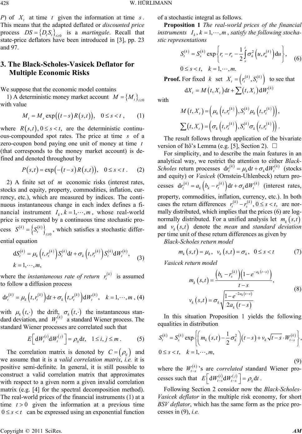

W. HÜRLIMANN 428
P) of t
X
at time t given the information at time
s
.
This means that the adapted deflated or discounted price
process

0
ttt
DSD S  is a martingale. Recall that
state-price deflators have been introduced in [3], pp. 23
and 97.
3. The Black-Scholes-Vasicek Deflator for
Multiple Economic Risks
We suppose that the economic model contains
1) A deterministic money market account


0
tt
MM


with value


 
exp,, 0
ts
M
MtsRst st , (1)
where

,,0 ,Rsts t are the deterministic continu-
ous-compounded spot rates. The price at time
s
of a
zero-coupon bond paying one unit of money at time t
(that corresponds to the money market account) is de-
fined and denoted throughout by
  
,exp ,,0Pstt sRstst . (2)
2) A finite set of m economic risks (interest rates,
stocks and equity, property, commodities, inflation, cur-
rency, etc.), which are measured by indices. The conti-
nuous instantaneous change in each index defines a fi-
nancial instrument ,1,,
k
I
km, whose real-world
price is represented by a continuous time stochastic pro-
cess
 

0
kk
tt
SS

, which satisfies a stochastic differ-
ential equation
 

 

 
d,d,d,
1,, ,
kkkkkk
tktt kttt
StrSttrSW
km
 

(3)
where the instantaneous rate of return
 k
t
r is assumed
to follow a diffusion process
 




d,d,d,1,,
kk kk
tktkt t
rtrttrWkm   , (4)
with


,
kt
  the drift,

,
kt


the instantaneous stan-
dard deviation, and

k
t
W a standard Wiener process. The
standard Wiener processes are correlated such that
 
dd d,1,
ij
tt ij
EW Wtijm 


 . (5)
The correlation matrix is denoted by


ij
C

 and
we assume that it is a valid correlation matrix, i.e. it is
positive semi-definite. In general, it is still possible to
construct a valid correlation matrix that approximates
with respect to a given norm a given invalid correlation
matrix (e.g. [4] for the spectral decomposition method).
The real-world prices of the financial instruments (1) at a
time 0t given the information at a previous time
0
s
t can be expressed using an exponentia l function
of a stochastic integral as follows.
Proposition 1 The real-world prices of the financial
instruments ,1,,
k
I
km

, satisfy the following stocha-
stic representations
 

2
1
exp,d ,
2
0,1,,.
t
kk k
tsts ku
s
SS rruru
st km







 


(6)
Proof. For fixed k set
 

,
kk
ttt
XrS to see that
 

d,d,d
k
tt tt
XMtXttXW

with




 



,,,,
kk k
tkttkt
MtXtr Str  ,




 



,,,,
kk k
tkttkt
tXtr Str  
.
The result follows through application of the bivariate
version of Itô’s Lemma (e.g. [5], Section 2). □
For simplicity, and to describe the main features in an
analytical way, we restrict the attention to either Black-
Scholes return processes
 
ddd
kk
tkkt
rtW   (stocks
and equity) or Vasicek (Ornstein-Uhlenbeck) return pro-
cesses
 



ddd
kkk
tkktkt
rabrt W    (interest rates,
property, commodities, inflation, currency, etc.). In both
cases the return differences
 
,0 ,
kk
ts
rr st are nor-
mally distributed, which implies that the prices (6) are log-
normally distributed. For a unified analysis let


,
k
mst
and


,
k
vst denote the mean and standard deviation
per time unit of these return differences as given by
Black-Scholes return model




,, ,, 0
kkkk
mst vstst 

 (7)
Vasicek return model









2
1
,,
1
,2
k
k
kats
ks
k
ats
kk
k
br e
mst ts
e
vst ats 






(8)
In this situation Proposition 1 yields the following
equalities in distribution
 
 
 2
1
exp ,,
2
0,1,,,
kk k
tskkk ts
SS msttsvtsW
st km











 
(9)
where the

k
ts
W

’s are correlated standard Wiener pro-
cesses such that
 
dd d
ij
ts tsij
EW Wt 




.
Following Section 2 consider now the Black-Scholes-
Vasicek deflator in the multiple risk economy, for short
BSV deflator, which has the same form as the price pro-
cesses in (9), i.e.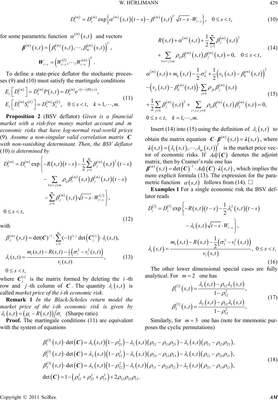

W. HÜRLIMANN 429
 
 



exp,,, 0,
T
mm mm
ts ts
DDsttssttsWst 

 (10)
for some parametric function


,
m
s
t  and vectors






 1
,,,,,
T
mm m
m
s
tst st  β,


1,, T
m
ts tsts
WW
 
W.
To define a state-price deflator the stochastic proces-
ses (9) and (10) must satisfy the martingale conditions
 

 
  
,
,,
,0, 1,,.
mm mtsRst
st ss
mk mk
stt ss
EDDPst De
EDSDSst km






 
(11)
Proposition 2 (BSV deflator) Given is a financial
market with a risk-free money market account and m
economic risks that have log-normal real-world prices
(9). Assume a non-singular valid correlation matrix C
with non-vanishing determinant. Then, the BSV deflator
(10) is determined by
 
 

 



 



2
1
1
1
1
exp ,,
2
,,
,,
0,
m
mm m
ts j
j
mm
ij ij
ijm
mmj
jts
j
DD Rsttsstts
s
tstts
sttsW
st

 






 











(12)
with



() 1()
1
22
1
2
,det()(1)det(,),
(,)(,)(,)
(,) ,
(,)
0,
m
miji
jji
i
iii
ii
s
tst
mstRstv st
st vst
st





 




CC
(13)
where

i
j
C is the matrix formed by deleting the i-th
row and j-th column of C. The quantity


,
i
s
t  is
called market price of the i-th economic risk.
Remark 1 In the Black-Scholes return model the
market price of the i-th economic risk is given by
  
,,
ii i
stR st

  (Sharpe ratio).
Proof. The martingale conditions (11) are equivalent
with the system of equations









2
1
1
1
,, ,
2
,,0,0,
m
mm
j
j
mm
ij ij
ijm
Rst stst
s
tst st

 

 




 (14)

 















2
2
2
,,
11
,,, ,
22
,,,
1,,,0,
2
0,1,,.
mm
kkkk
mm
kk jkj
jk
mmm
jijij
jk ijijk
s
tmstvstst
vst stst
stst st
st km






 


 



(15)
Insert (14) into (15) using the definition of


,
i
s
t  to
obtain the matrix equation

 
,,
m
s
tstCβλ, where
 

1
,,,,,
T
m
s
tst st  λ is the market price vec-
tor of economic risks. If

Adj C denotes the adjoint
matrix, then by Cramer’s rule one has

 
1
,det ,
m
s
tAdjst

βCCλ, which implies the
more explicit formula (13). The expression for the para-
metric function


,
s
t 
follows from (14). □
Examples 1 For a single economic risk the BSV def-
lator reads
 
  

  


11 2
1
1
22
111
11
1
exp ,,
2
,,
1
,, ,
2
,, 0,
,
ts
ts
D DRsttsstts
stt sW
mstRstv st
s
tst
vst






 









(16)
The other lower dimensional special cases are fully
analytical. For 2m

one has





  
21122
12
12
22121
22
12
,,
,,
1
,,
,,
1
s
tst
st
s
tst
st








(17)
Similarly, for 3m

one has (note for mnemonic pur-
poses the cyclic permutations)

 

   

 






 

   


32
112321213 2331312 23
32
221332312 1311223 13
32
331211323 1222313 12
222
1223131223 13
,det ,1,,,
,det ,1,,,
,det ,1,,,
det 12
st st stst
stst stst
stst stst
 

 
 
 
 
 
 
C
C
C
C.
(18)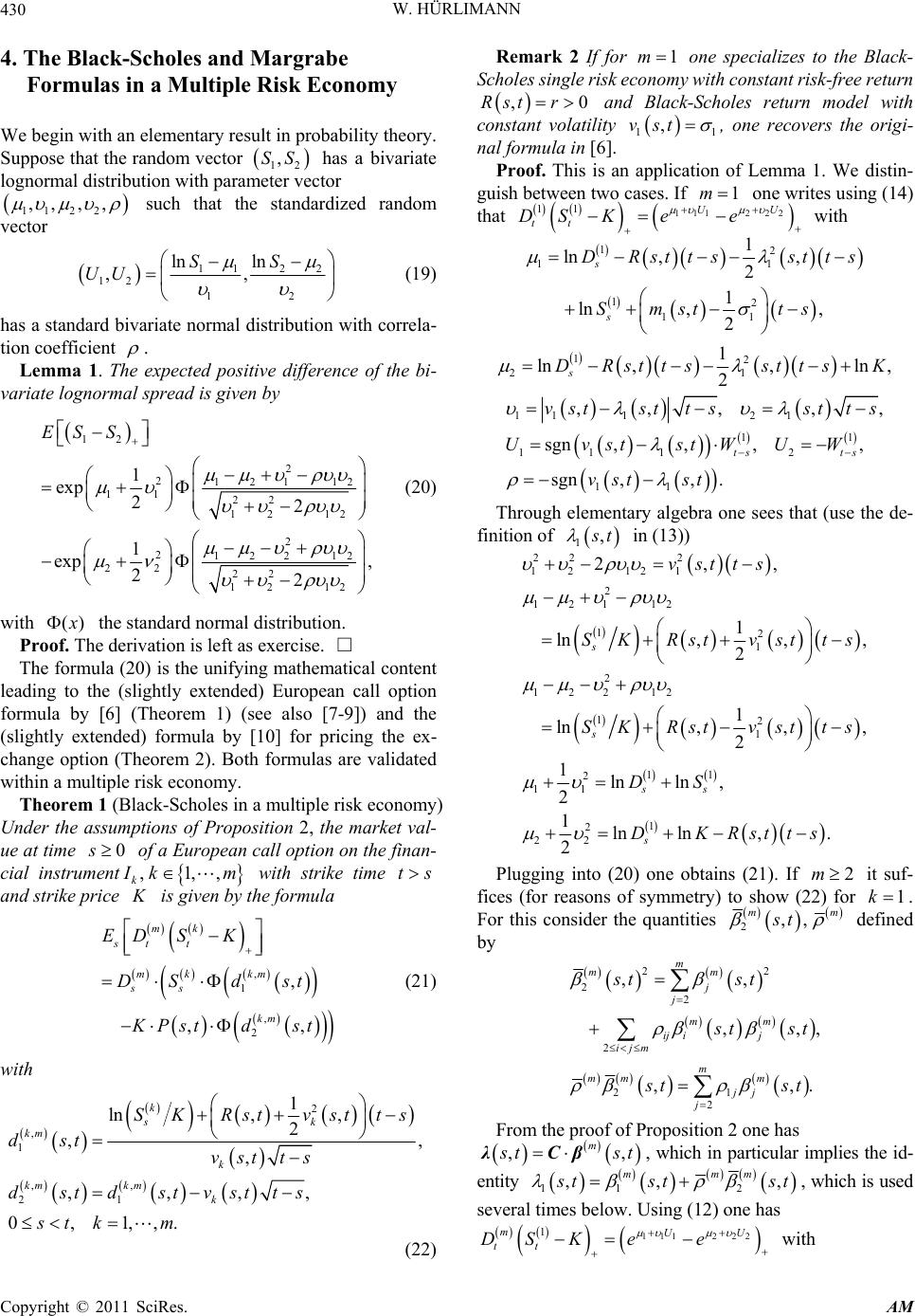

W. HÜRLIMANN 430
4. The Black-Scholes and Margrabe
Formulas in a Multiple Risk Economy
We begin with an elementary result in probability theory.
Suppose that the random vector

12
,SS has a bivariate
lognormal distribution with parameter vector

112 2
,, ,,

 such that the standardized random
vector

112 2
12 12
ln ln
,,
SS
UU







(19)
has a standard bivariate normal distribution with correla-
tion coefficient

.
Lemma 1. The expected positive difference of the bi-
variate lognorma l spread is given by

12
2
2121 12
11 22
12 12
2
2122 12
22 22
12 12
1
exp 22
1
exp ,
22
ES S
 
 
 
  























(20)
with )(x the standard normal distribution.
Proof. The derivation is left as exercise. □
The formula (20) is the unifying mathematical content
leading to the (slightly extended) European call option
formula by [6] (Theorem 1) (see also [7-9]) and the
(slightly extended) formula by [10] for pricing the ex-
change option (Theorem 2). Both formulas are validated
within a multiple risk economy.
Theorem 1 (Black-Scholes in a multiple risk economy)
Under the assumptions of Proposition 2, the market val-
ue at time 0s of a European call option on the finan-
cial instrument

,1,,
k
I
km with strike time ts
and strike price K is give n by the for m ula
 










,
1
,
2
,
,,
mk
st t
mk km
ss
km
ED SK
DSdst
K
Pst d st






 
(21)
with




  




 
2
,
1
,,
21
1
ln, ,
2
,,
,
,,,,
0,1,,.
k
sk
km
k
kmkm k
SK Rstvstts
dst vst ts
dstdstvstts
st km

 




 
(22)
Remark 2 If for 1m

one specializes to the Black-
Scholes single risk economy with constant risk-free return


,0Rst r

 and Black-Scholes return model with
constant volatility


11
,vst


, one recovers the origi-
nal formula in [6].
Proof. This is an application of Lemma 1. We distin-
guish between two cases. If 1m one writes using (14)
that
 




1112 22
11 UU
tt
DS Kee
  


  with

  

 
12
11
12
11
1
ln ,,
2
1
ln ,,
2
s
s
DRst tsstt s
Smst ts





 



  
12
21
1
ln,,ln ,
2
s
DRst tssttsK  
 
  
 
 

11 121
11
111 2
11
,,, ,,
sgn ,,,,
sgn,,.
ts ts
vststtsst ts
Uv ststWUW
vst st
 






 
Through elementary algebra one sees that (use the de-
finition of


1,
s
t  in (13))

 


 


 
 

 
22 2
12 121
2
121 12
12
1
2
122 12
12
1
11
2
11
1
2
22
2,,
1
ln,, ,
2
1
ln,, ,
2
1lnln ,
2
1ln ln,.
2
s
s
ss
s
vstts
SK Rstvstts
SK Rstvstts
DS
DKRstts
 
 



 


 




 


 
 
Plugging into (20) one obtains (21). If 2m it suf-
fices (for reasons of symmetry) to show (22) for 1k

.
For this consider the quantities



2,,
mm
st

defined
by








 



22
22
2
21
2
,,
,,,
,,.
m
mm
j
j
mm
ij ij
ijm
m
mm m
jj
j
st st
s
tst
s
tst


 

 







From the proof of Proposition 2 one has



,,
m
s
tstλCβ, which in particular implies the id-
entity



 

11 2
,, ,
mmm
s
tst st    , which is used
several times below. Using (12) one has
 




1112 22
1mUU
tt
DS Kee
  


  with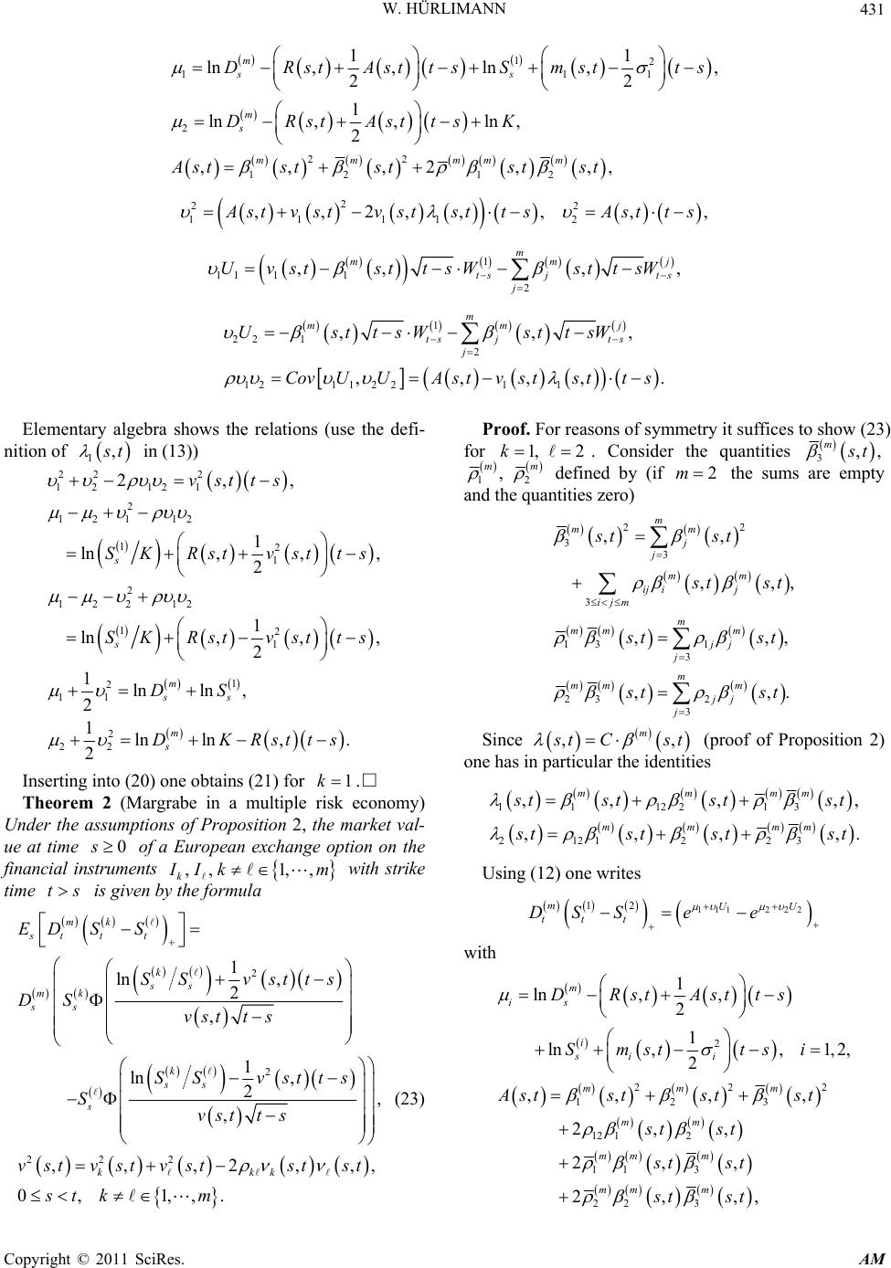

W. HÜRLIMANN 431

  

 

  





 



12
111
2
22
12 12
11
ln, ,ln,,
22
1
ln,,ln ,
2
,, ,2,,,
m
ss
m
s
mm mmm
DRstAsttsSmst ts
DRstAsttsK
Astststst st


 

 



 



 

 
2
2 2
1111 2
,,2,,, ,,
A
stvstvststt sAstt s   




 


1
11 112
,,, ,
m
mmj
ts jts
j
Uvststt sWsttsW  


 



 






1
22 12
121 12211
,,,
,,,,.
m
mmj
ts jts
j
UsttsWsttsW
CovUUAstvs ts tts
 
 


 


Elementary algebra shows the relations (use the defi-
nition of


1,
s
t  in (13))
 


 


 
 

 
22 2
12 121
2
121 12
12
1
2
122 12
12
1
1
2
11
2
22
2,,
1
ln,, ,
2
1
ln,, ,
2
1lnln ,
2
1ln ln,.
2
s
s
m
ss
m
s
vstts
SK Rstvstts
SK Rstvstts
DS
DKRstts
 
 



 


 




 


 
 
Inserting into (20) one obtains (21) for 1k.□
Theorem 2 (Margrabe in a multiple risk economy)
Under the assumptions of Proposition 2, the market val-
ue at time 0s of a European exchange option on the
financial instruments

,, 1,,
k
I
Ik m

with strike
time ts is given by the formula
 

 
 

 


 

 



2
2
222
1
ln ,
2
,
1
ln ,
2
,
,
,,,2,,,
0, 1,,.
mk
st tt
k
ss
mk
ss
k
ss
s
kkk
ED SS
SS vstts
DS vstt s
SS vstts
Svstt s
vstvst vststst
st km
 




















 








 






(23)
Proof. For reasons of symmetry it suffices to show (23)
for 1, 2k

. Consider the quantities


3,,
m
s
t 
 
12
,
mm

 defined by (if 2m the sums are empty
and the quantities zero)








 



 



22
33
3
13 1
3
23 2
3
,,
,,,
,,,
,,.
m
mm
j
j
mm
ij ij
ijm
m
mm m
jj
j
m
mm m
jj
j
st st
s
tst
s
tst
s
tst


 
 

 










Since



,,
m
s
tC st   (proof of Proposition 2)
one has in particular the identities





 






 

1112213
2121 2 23
,, ,,,
,,,,.
mmmm
mmmm
s
tst stst
s
tstst st
  



Using (12) one writes
 



1112 22
12mUU
tt t
DS See
  


 
with

  

 











 



 



2
222
123
12 12
11 3
22 3
1
ln, ,
2
1
ln,, 1,2,
2
,, , ,
2,,
2,,
2,,,
m
is
i
si i
mmm
mm
mm m
mm m
DRstAstts
Smst tsi
Ast ststst
st st
st st
st st



 



 



 







W. HÜRLIMANN 432
 


 









 













2
2
1111
2
2
2222
1
11 11
2
23
1
22 1
2
22
3
12
,,2,, ,
,,2,, ,
,,
,,,
,
,,
,,
mts
m
mmj
ts jts
j
mts
mts
mmj
jts
j
A
stv stv ststts
A
stvstv ststt s
Uv ststtsW
stt sWsttsW
UsttsW
vstst tsW
stt sW
Cov







 







 
 
 

 
 





  
  
112 2
112 2
12 12
,
,,,,,
,,.
UU
Ast vstst vstst
vstvst ts



 

One obtains the relations (use again the definition of

,, 1,2
ist i
  in (13))
 


 
 

 
 

 
 
22
12 12
22
12 1212
2
2
121 12
12 2
2
122 12
12 2
2
2
,,2,,
,,
1
ln, ,
2
1
ln, ,
2
1lnln ,1,2.
2
ss
ss
mi
ii ss
v stv stststt s
vst ts
SS vstts
SS vstts
DSi
 
 
 



 





 
Inserting into (20) one obtains the Formula (23) for
1, 2k.□
It might be useful to conclude with a short summary.
If one starts with the stochastic representation (9) of the
real-world prices for the risks in the economy, the deri-
vation of the formulas is rather elementary. It only uses
introductory Probability Theory (including the notion of
Martingale) and Linear Algebra. Therefore, the proof is
accessible to any knowledgeable person in these mathe-
matical areas. Moreover, the approach is different from
the original one (hedging argument, use of Itô’s Lemma
and solution of a partial differential equ ation). It leads to
new insight in Option Pricing Theory. Besides a general
validation in a multiple risk economy, the proposed de-
rivation implies a risk-neutral property of independent
interest, i.e. the formulas are invariant with respect to the
market prices of the risk factors.
5. References
[1] R. C. Merton, “Theory of Rational Option Pricing,” Bell
Journal of Economics and Management Science, Vol. 4,
No. 8, 1973, pp. 141-183. Reprinted in [2].
doi:10.2307/3003143
[2] R. C. Merton, “Continuous-Time Finance,” Basil Black-
well, 1990.
[3] D. Duffie, “Dynamic Asset Pricing Theory,” Princeton
University Press, New Jersey, 1992.
[4] R. Rebonato and P. Jäckel, “The Most General Metho-
dology to Create a Valid Correlation Matrix for Risk
Management and Option Pricing Purposes,” Journal of
Risk, Vol. 2, No. 2, 2000, pp. 17-27.
[5] W. Hürlimann, “Méthodes Stochastiques D'évaluation du
Rendement,” Proceedings of the 3rd International AFIR
Colloquium, Rom, Vol. 2, 1993, pp. 629-649.
[6] F. Black and M. Scholes, “The Pricing of Options and
Corporate Liabilities,” Journal of Political Economy, Vol.
81, No. 3, 1973, pp. 637-59. Reprinted in [7-9].
doi:10.1086/260062
[7] M. C. Jensen (Editor), “Studies in the Theory of Capital
Market,” Praeger, New York, 1972.
[8] D. L. Luskin (Editor), “Portfolio Insurance: A Guide to
Dynamic Hedging,” John Wiley, New York, 1988.
[9] L. Hugston (Editor), “Options: Classic Approaches to
Pricing and Modelling,” Risk Books, London, 1999.
[10] W. Margrabe, “The Value of an Option to Exchange one
Asset for Another,” Journal of Finance, Vol. 33, No. 1,
pp. 177-186, 1978. Reprinted in [9].
doi:10.2307/2326358