Paper Menu >>
Journal Menu >>
 Applied Mathematics, 2011, 2, 414-423 doi:10.4236/am.2011.24051 Published Online April 2011 (http://www.SciRP.org/journal/am) Copyright © 2011 SciRes. AM RBFs Meshless Method of Lines for the Numerical Solution of Time-Dependent Nonlinear Coupled Partial Differential Equations Sirajul Haq1, Arshad Hussain1, Marjan Uddin2,3* 1Faculty of Engineering Sciences, Ghulam Ishaq Khan Institute of Engineering Sciences and Technology, Topi, Pakistan 2Department of Applied Mathematics, Illinois Institute of Technology, Chicago, USA 3Department of Mathematics, Karakoram International University, Gilgit, Pakistan E-mail: siraj_jcs@yahoo.co.in, math_pal@hotmail.com, marjankhan1@hotmail.com* Received December 25, 2010; revised February 3, 2011; accepted February 6, 2011 Abstract In this paper a meshless method of lines is proposed for the numerical solution of time-dependent nonlinear coupled partial differential equations. Contrary to mesh oriented methods of lines using the finite-difference and finite element methods to approximate spatial derivatives, this new technique does not require a mesh in the problem domain, and a set of scattered nodes provided by initial data is required for the solution of the problem using some radial basis functions. Accuracy of the method is assessed in terms of the error norms L2, L∞ and the three invariants C1, C2, C3. Numerical experiments are performed to demonstrate the accuracy and easy implementation of this method for the three classes of time-dependent nonlinear coupled partial diffe- rential equations. Keywords: RBFs, Meshless Method of Lines, Time-Dependent PDEs 1. Introduction Nonlinear coupled partial differential equations have nu- merous applications in the field of science and engineer- ing, including solid state physics, fluid mechanics, che- mical physics, plasma physics etc. (see [1-3] and the ref- erences therein). In 1981 Hirota-Satsuma introduced the coupled KdV equations, [4] which has many applications in physical sciences. Coupled KdV equations describe an interaction of the two long waves with different disper- sion relation. The Burgers’ equations describe phenomena such as a mathematical model of turbulence [5] and the nonlinear hyperbolic system [6] represents interaction of the two waves traveling in the opposite directions. In the last decade many authors have studied the nu- merical and approximate solution of time-dependent nonlinear coupled partial differential equations by vari- ous numerical methods. These include Adomian decom- position method [7], the local discontinuous Galerkin method [8], the variational iteration method [9], the Chebyshev spectral collocation method [10] and the radial basis functions method [6,11,12]. In the last decade, the theory of radial basis functions (RBFs) has enjoyed a great success as scattered data in- terpolating technique. A radial basis function, jj x xxx , is a continuous spline which de- pends upon the separation distances of a subset of data centers, n X , ,1,2,, j x Xj N. Due to sphe- rical symmetry about the centers j x , the RBFs are called radial. The distances, j x x, are usually taken to be the Euclidean metric. Hardy [13] was the first to introduced a general scat- tered data interpolation method, called radial basis func- tions method for the approximation of two-dimensional geographical surfaces. In 1982 Franke [14] in a review paper made the comparison among all the interpolation methods for scattered data sets available at that time, and the radial basis functions outperformed all the other me- thods regarding efficiency, stability and ease of imple- mentations. Franke found that Hardy’s multiquadrics (MQ) were ranked the best in accuracy, followed by thin plate splines (TPS). Despite MQ’s excellent performance, it contains a shape parameter c, and the accuracy of MQ is greatly affected by the choice of shape parameter c whose optimal value is still unknown. Franke [15] used the formula 2 22 1.25cd where d is the mean dis-  S. HAQ ET AL. Copyright © 2011 SciRes. AM 415 tance from each data point to its nearest neighbor. Hick- ernell and Hon [16] and Golberg et al. [17] had success- fully used the technique of cross-validation to obtain an optimal value of the shape parameter. Various research- ers have contributed recently to this field (see [18-25] ect.) The method of lines (MOL) [26] is a general proce- dure for the solution of time dependent partial differen- tial equations (PDEs). The basic idea of the MOL is to replace the spatial (boundary value) derivatives in the PDEs with algebraic approximations. Once this is done, the spatial derivatives are no longer stated explicitly in terms of the spatial independent variables. Thus only the initial value variable, typically time in a physical prob- lem, remains. In other words, we have a system of ODEs that approximate the original PDE. Now we can apply any integration algorithm for initial value ODEs to com- pute an approximate numerical solution to the PDE. Thus, one of the salient features of the MOL is the use of ex- isting, and generally well established, numerical methods for ODEs. Very recently Quan Shen [27] use this ap- proach for the numerical solution of KdV equation. In this paper, we will use RBFs approximation method with the method of lines (MOL) for the numerical solution of time-dependent nonlinear partial differential equations given as: Class A: Coupled KdV equations 62, txxx xx uu uuvv 3, txxx x vv uv Class B: Coupled Burgers’ equations 2, txx x x u uuuuv 2, txx x x vv vvuv Class C: System of nonlinear hyperbolic equations , tx uuuv , tx vv uv where ,, are positive parameters. Rest of the paper is organized as follows: In Section 2, The radial basis functions collocation method coupled with MOL is presented. Section 3 is devoted to the nu- merical tests of the method on the problems related to the coupled KdV, the coupled Burgers’ equations and the system of nonlinear hyperbolic equations. In Section 4, the results are concluded. 2. RBFs Meshless Method of Lines 2.1. Coupled KdV Equations Consider the nonlinear coupled KdV equations, 62, 3, t xxxxx t xxxx uu uuvv vv uv (1) with boundary conditions 12 12 ,, ,, ,,,,0, uat ftubt ft vatgtvbt gtt (2) and initial conditions ,0 , ,0 ,, uxfx vxgx ax b (3) where ,, are positive real constants. For a given set of N collocation points 1 N ii x in the domain ,ab, the RBFs approximation for u and v of (1) are given by 12 11 ,, NN jj jj Uxr Vxr (4) where 1 N j j are the unknown constants to be deter- mined, j j rxx can be any well known ra- dial basis function and j j rxx is the Euclidean norm between points x and . j x Here we are using two radial basis functions, the multiquadric 22 rrc and cubic 3.rr Now for each node , 1,2,3,, i x iN in the domain ,ab , (4) can be written as 12 ,, UAVA (5) where 123 ,,,, T N Ux UxUxUx U 123 ,,,,, 1,2. T ii iiNi i 11 211 1 12 12 1 11 T N T T NN NN N x xx x xx x xx x x A 123 ,,,, , T iiiiNi xxxxx where 1,2, 3,,iN . Equation (4) can also be written as 1 1 , T T Ux x Vx x A UDxU A VDxV (6) where 1 12 ,,, . T N x DxD xDx Dx A Using the approximations i Ut and i Vt of the  S. HAQ ET AL. Copyright © 2011 SciRes. AM 416 solutions , i uxt and , i vxt given in (6), (1) at each node , 1,2,3,, i x iN can be written as d6 d 2 d3 d i xxx iix i ixi i xxx iix i UDx UDx t VD x VDx UDx t UU V VV (7) where 12 ,,, , ixixiNxi DxD xDx x Dx ,1,2,,, jx ij i DxDxjN x 12 ,,, ixxx ixxx iNxxx i DxDxDx xxx Dx 3 3,1,2,,. jxxx iji DxDxjN x In more compact form (7) can be written as d62, d d3, d xxx xx xxx x t t U D UUDU VDV VDVU DV (8) where the symbol * denotes component by component multiplication of two vectors and ,1 ,1 ,. NN xjxi xxxjxxxi ij ij DxD x DD For simplicity we write (8) as 12 dd ,, ,, dd FF tt UV UVUV (9) where 1,62, xxx xx F UVD UUDUVDV 2,3. xxx x F UVD VUDV The corresponding boundary conditions are given by 11 2 11 2 , ,, N N UftU ft VgtVgt (10) and the initial conditions are as 012 012 ,,, ,,, N N tfxfx fx tgxgxgx U V (11) Now we solve the system of ODEs (9)-(11) by using the well known ODE solvers. 1) The classical forth order Runge-Kutta method (RK4) given by 1 12 34 δ22 , 6 nn tKK KK UU 1 1234 22 , 6 nn t J JJJ VV where 1121 1 ,, 2,, nnn n KFK FtKUVUV 31 241 3 δ2, ,, , nn nn K FtKKFtK UV UV 12 221 ,,, 2, nn nn JFJ FtJUVUV 322 423 ,δ2,, δ, nn nn J FtJJFtJ UVUV 2) Low-storage third-order (TVD-RK3) scheme given by [28] 1 1 δ,, nnn tFUU UV 211 1 31 1 δ,, 44 4 nn tF UUU UV 122 1 12 2 δ,, 333 nnn tF UUU UV 1 2 δ,, nnn tFVV UV 21 1 2 31 1 δ,, 44 4 nn tF VVV UV 12 2 2 12 2 δ,. 33 3 nnn tF VVV UV 2.2. Nonlinear Coupled Burgers’ Equations Consider the nonlinear coupled Burgers’ equations 2, 2, txx x x txx xx u uuuuv vv vvuv (12) with the boundary conditions 12 12 ,, ,, ,,,,0, uat ftubt ft vatgtvbt gtt (13) and initial conditions ,0 , ,0 ,, uxfx vxgx ax b (14) where ,, are positive parameters. The same proce- dure as discussed in Section 2.1 can be used for the solu- tion of (12)-(14). 2.3. Nonlinear Coupled Hyperbolics Consider the nonlinear hyperbolic system ,, tx tx uuuv vvuv (15) with boundary conditions  S. HAQ ET AL. Copyright © 2011 SciRes. AM 417 12 12 ,,, , ,,,,0, uat ftubt ft vatgtvbt gtt (16) and initial conditions ,0 , ,0 ,, uxfx vxgxaxb (17) where is a positive real constant. The same proce- dure as discussed in Section 2.1 can be used for the solu- tion of (15)-(17). 3. Numerical Examples In this section, we apply the RBFs meshless method of lines for the numerical solution of three classes of partial differential equations, defined earlier. We use the 2 L and L error norms to measure the difference between the numerical and analytic solutions. The 2 L and L error norms of the solution are defined by 12 2 221 δ, max , N j j LuU xuU LuU uU (18) We examine our results by calculating the following three conservative laws. Hirota-Satsuma [4] proved that the coupled KdV equations defined in (1) possesses three conserved quantities for all values of and . 1 22 2 22 32 3 d, 2d 3 1 1d. 2 b a b a b xx a Cux Cu vx Cauuuvvx (19) Later Hirota-Satsuma [29] showed that the system (7) has infinitely many conserved quantities for the choice of 12 and arbitrary values of and . In our in- vestigation we consider the conserved quantities 1,C 2 C and 3 C only. In this section, we apply meshless MOL using radial basis functions on the three classes of partial differential equations defined earlier. Problem 1 We consider the nonlinear coupled KdV Equations (1) for v = 3 α = β and with exact solution [20] 2 2 1 ,sec , 2 1 ,sec. 2 2 uxthx t vxthx t (20) where , are arbitrary constants. The boundary con- ditions ,,uat ,,ubt ,vat and ,vbt and the initial conditions ,0 ,,0uxvx are extracted from the exact solution (20). We solved the problem in the spatial interval 55x by RBFs meshless method of lines using RK4 and TVD-RK3 time integration schemes. In our computations we used multiquadric (MQ) radial ba- sis function. The results are presented in Tables 1-4, and in Figure 1. It is observed that the two schemes RK4 and TVD-RK3 show same order of accuracy, but TVD-RK3 scheme is more faster than RK4 scheme, and both re- mained stable for small time step size δt It is also ob- served that the three invariants 1,C 2 C and 3 C as well as their normalized values, 11 11 00,NCC tCC 22 22 00,NCC tCC 33 33 00,NCC tCC are absolutely conserved in time during the computations which demonstrates the accuracy of the schemes. We also noted that the value of MQ shape parameter for which the solution converges belongs to the interval 0.1 0.6c as shown in Table 3. The motion of solitary waves u and v is shown in Figure 1, which are initially centered at 0x moving from left to right with the constant speed , having the amplitudes and2 respectively. Problem 2 Consider the nonlinear coupled Burgers’ Equations (12), whose exact solution [10] is given by 0 0 21 ,2 tanh2, 41 21 21 ,2tanh2. 2141 uxtaAAxAt vxt aAAx At (21) where 0 12412 1,Aa 0,a , are arbitrary constants. The boundary conditions ,,uat ,,ubt ,,vat ,vbt and the initial conditions ,0 ,ux ,0vx are extracted from the exact solution (21). We solved the problem in the domain 10 10x by using MOL coupled with RBFs collocation method. The classical RK4 and TVD-RK3 scheme are used in our computa- tions. The results are listed in Table 5 and Figure 2, and compare with earlier results [10]. It is observed that the results are comparable with [10] and well agreed with the exact solution. Problem 3 Now we consider nonlinear coupled hyper- bolic Equations (15). For the sake of comparison [6], we take 0.5,a 0.5,b 100 and the initial condi- tions.  S. HAQ ET AL. Copyright © 2011 SciRes. AM 418 (a) (b) (c) (d) Figure 1. Plots of Problem 1 corresponding to α = 0.1, β = 0.1, λ = 0.5, δx = 0.1, δt = 0.001, c = 0.58. Figures 1(a) and 1(b) show the motion of the solitary waves u and v moving from left to right, initially centered at x = 0 when t = 0,1,2,3,4,5. Figures 1(c) and 1(d) represent numerical solutions u and v over time [0,5]. 0.51cos10,0.3,0.1; ,0 0, otherwise xx ux (22) 0.51cos10,0.1,0.3 ; ,0 0, otherwise xx vx (23) and the boundary conditions ,,0, ,,0. uat ubt vat vbt (24) This problem is solved by RBFs meshless method of lines using MQ with RK4 scheme. We take the initial so- lutions v and ,0vx which are located at 0.2x and 0.2,x respectively. When 0t the nonlinear term, uv , causes these waves to move without change in shape, u to the right and v to the left. The two waves collide when 0.1t which results in change of shapes of the waves. The two waves overlap each other near 0.25t and they separate again at 0.3t approx- imately. From this time onwards the linear term becomes dominant and the pulses lose their symmetry and expe- rience a decrease in the amplitude due to nonlinear inte- raction as shown in the Figures 3 (a)-3(f). The numerical results of the solutions u and v are presented graphi- cally. Since the exact solution of this problem is not known, we use cubic radial basis function 3 r to find the numerical solution. These graphical results are agreed well with the results obtained by quasi-linear interpola- tion method [6]. 4. Closure We have applied the meshless method of lines using radial basis functions for the numerical solutions of time- dependent nonlinear coupled partial differential equa- 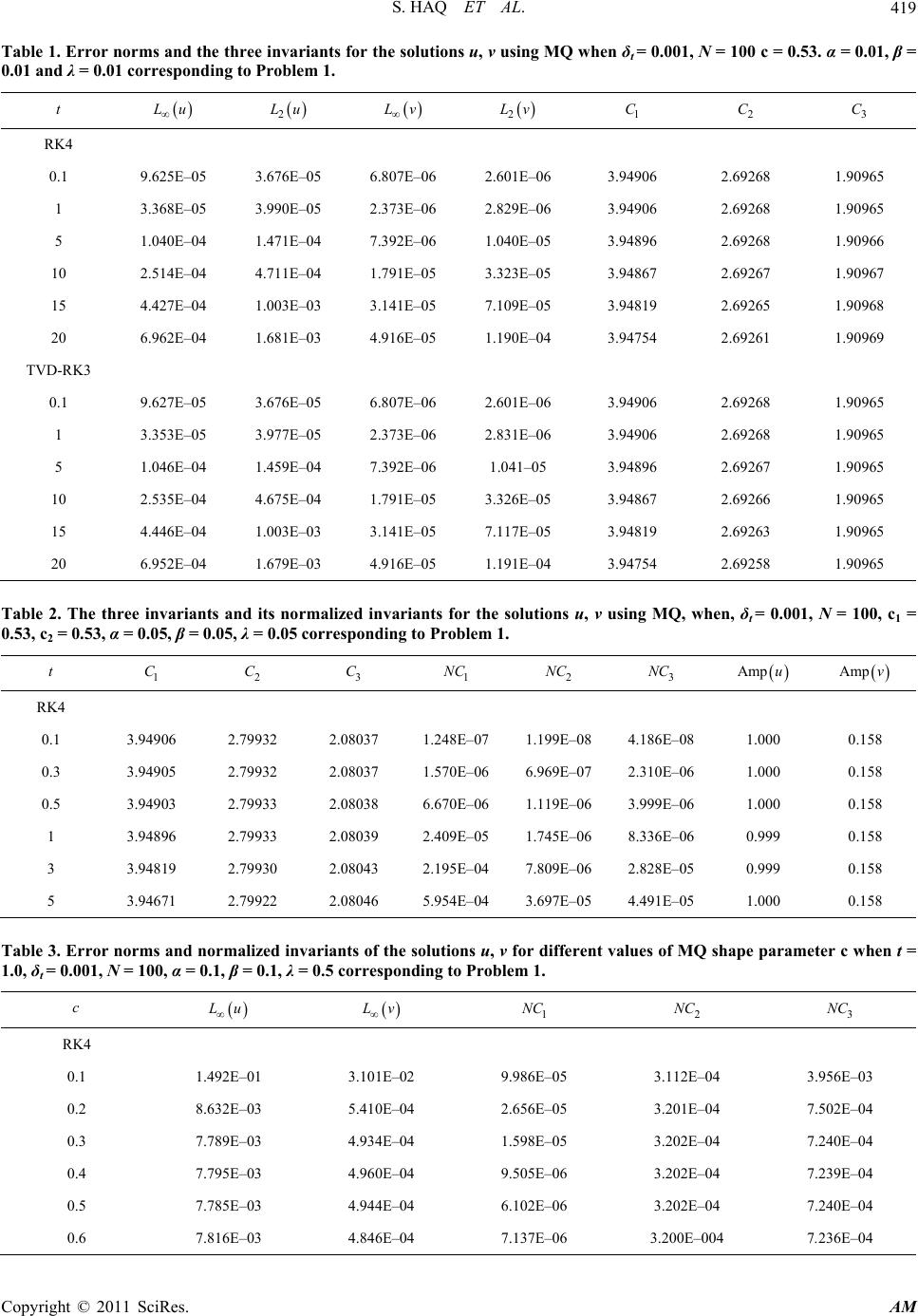 S. HAQ ET AL. Copyright © 2011 SciRes. AM 419 Table 1. Error norms and the three invariants for the solutions u, v using MQ when δt = 0.001, N = 100 c = 0.53. α = 0.01, β = 0.01 and λ = 0.01 corresponding to Problem 1. t L u 2 L u L v 2 L v 1 C 2 C 3 C RK4 0.1 9.625E–05 3.676E–05 6.807E–06 2.601E–06 3.94906 2.69268 1.90965 1 3.368E–05 3.990E–05 2.373E–06 2.829E–06 3.94906 2.69268 1.90965 5 1.040E–04 1.471E–04 7.392E–06 1.040E–05 3.94896 2.69268 1.90966 10 2.514E–04 4.711E–04 1.791E–05 3.323E–05 3.94867 2.69267 1.90967 15 4.427E–04 1.003E–03 3.141E–05 7.109E–05 3.94819 2.69265 1.90968 20 6.962E–04 1.681E–03 4.916E–05 1.190E–04 3.94754 2.69261 1.90969 TVD-RK3 0.1 9.627E–05 3.676E–05 6.807E–06 2.601E–06 3.94906 2.69268 1.90965 1 3.353E–05 3.977E–05 2.373E–06 2.831E–06 3.94906 2.69268 1.90965 5 1.046E–04 1.459E–04 7.392E–06 1.041–05 3.94896 2.69267 1.90965 10 2.535E–04 4.675E–04 1.791E–05 3.326E–05 3.94867 2.69266 1.90965 15 4.446E–04 1.003E–03 3.141E–05 7.117E–05 3.94819 2.69263 1.90965 20 6.952E–04 1.679E–03 4.916E–05 1.191E–04 3.94754 2.69258 1.90965 Table 2. The three invariants and its normalized invariants for the solutions u, v using MQ, when, δt = 0.001, N = 100, c1 = 0.53, c2 = 0.53, α = 0.05, β = 0.05, λ = 0.05 corresponding to Problem 1. t 1 C 2 C 3 C 1 NC 2 NC 3 NC Amp u Amp v RK4 0.1 3.94906 2.79932 2.08037 1.248E–07 1.199E–08 4.186E–08 1.000 0.158 0.3 3.94905 2.79932 2.08037 1.570E–06 6.969E–07 2.310E–06 1.000 0.158 0.5 3.94903 2.79933 2.08038 6.670E–06 1.119E–06 3.999E–06 1.000 0.158 1 3.94896 2.79933 2.08039 2.409E–05 1.745E–06 8.336E–06 0.999 0.158 3 3.94819 2.79930 2.08043 2.195E–04 7.809E–06 2.828E–05 0.999 0.158 5 3.94671 2.79922 2.08046 5.954E–04 3.697E–05 4.491E–05 1.000 0.158 Table 3. Error norms and normalized invariants of the solutions u, v for different values of MQ shape parameter c when t = 1.0, δt = 0.001, N = 100, α = 0.1, β = 0.1, λ = 0.5 corresponding to Problem 1. c L u L v 1 NC 2 NC 3 NC RK4 0.1 1.492E–01 3.101E–02 9.986E–05 3.112E–04 3.956E–03 0.2 8.632E–03 5.410E–04 2.656E–05 3.201E–04 7.502E–04 0.3 7.789E–03 4.934E–04 1.598E–05 3.202E–04 7.240E–04 0.4 7.795E–03 4.960E–04 9.505E–06 3.202E–04 7.239E–04 0.5 7.785E–03 4.944E–04 6.102E–06 3.202E–04 7.240E–04 0.6 7.816E–03 4.846E–04 7.137E–06 3.200E–004 7.236E–04 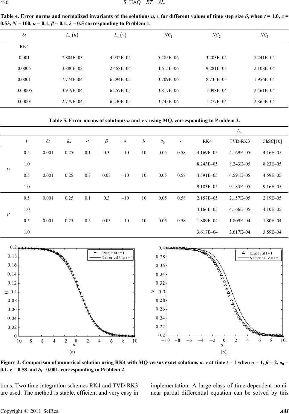 S. HAQ ET AL. Copyright © 2011 SciRes. AM 420 Table 4. Error norms and normalized invariants of the solutions u, v for different values of time step size δt when t = 1.0, c = 0.53, N = 100, α = 0.1, β = 0.1, λ = 0.5 corresponding to Problem 1. δt L u L v 1 NC 2 NC 3 NC RK4 0.001 7.804E–03 4.932E–04 5.485E–06 3.203E–04 7.241E–04 0.0005 3.880E–03 2.458E–04 4.615E–06 9.281E–05 2.108E–04 0.0001 7.774E–04 6.294E–05 3.709E–06 8.735E–05 1.956E–04 0.00005 3.919E–04 6.257E–05 3.817E–06 1.098E–04 2.461E–04 0.00001 2.779E–04 6.230E–05 3.745E–06 1.277E–04 2.865E–04 Table 5. Error norms of solutions u and v v using MQ, corresponding to Problem 2. L t δt δ x a b 0 a c RK4 TVD-RK3 ChSC[10] U 0.5 0.001 0.25 0.1 0.3 –10 10 0.05 0.58 4.169E–05 4.169E–05 4.16E–05 1.0 8.243E–05 8.243E–05 8.23E–05 0.5 0.001 0.25 0.3 0.03 –10 10 0.05 0.58 4.591E–05 4.591E–05 4.59E–05 1.0 9.183E–05 9.183E–05 9.16E–05 V 0.5 0.001 0.25 0.1 0.3 –10 10 0.05 0.58 2.157E–05 2.157E–05 2.19E–05 1.0 4.166E–05 4.166E–05 4.10E–05 0.5 0.001 0.25 0.3 0.03 –10 10 0.05 0.58 1.809E–04 1.809E–04 1.80E–04 1.0 3.617E–04 3.617E–04 3.59E–04 (a) (b) Figure 2. Comparison of numerical solution using RK4 with MQ versus exact solutions u, v at time t = 1 w hen α = 1, β = 2, a0 = 0.1, c = 0.58 and δt =0.001, corresponding to Problem 2. tions. Two time integration schemes RK4 and TVD-RK3 are used. The method is stable, efficient and very easy in implementation. A large class of time-dependent nonli- near partial differential equation can be solved by this  S. HAQ ET AL. Copyright © 2011 SciRes. AM 421 (a) (b) (c) (d) (e) (f) Figure 3. Numerical solution using quintics. Figures 3(a)-3(f) show the motion and interaction of the waves u and v.  S. HAQ ET AL. Copyright © 2011 SciRes. AM 422 technique. 5. Acknowledgements The work presented in this paper is supported by HEC Pakistan through grants 063-281079-Ps3-169, IRSIP 14 Ps3. 6. References [1] A. Osborne, “The Inverse Scattering Transform: Tools for the Nonlinear Fourier Analysis and Filtering of Ocean Surface Water Waves,” Chaos. Solitons & Fractals, Vol. 5, No. 12, 1995, pp. 2623-37. doi:10.1016/0960-0779(94)E0118-9 [2] L. Ostrovsky and Y. A. Stepanyants, “Do Internal Solu- tions Exist in the Ocean,” Reviews of Geophysics, Vol. 27, No. 3, 1989, pp. 293-310. doi:10.1029/RG027i003p00293 [3] G. C. Das and J. Sarma “Response to ‘Comment on’ a New Mathematical Approach for Finding the Solitary Waves in Dusty Plasma,” Physics of Plasmas, Vol. 6, No. 11, 1999, pp. 4394-4397. doi:10.1063/1.873705 [4] R. Hirota and J. Satsuma, “Soliton Solutions of a Coupled Kortewege-de Vries Equation,” Physics Letters A, Vol. 85, No. 8-9, 1981, pp. 407-408. doi:10.1016/0375-9601(81)90423-0 [5] Y. C. Hon and X. Z. Mao, “An Efficient Numerical Scheme for Burgers Equation,” Applied Mathematics and Computation, Vol. 95, No. 1, 1998, pp. 37-50. doi:10.1016/S0096-3003(97)10060-1 [6] R. Chen and Z. Wu, “Solving Partial Differential Equa- tion by Using Multiquadric Quasiinterpolation,” Applied Mathematics and Computation, Vol. 186, No. 2, 2007, pp. 1502-1510. doi:10.1016/j.amc.2006.07.160 [7] D. Kaya and E. I. Inan, “Exact and Numerical Traveling Wave Solutions for Nonlinear Coupled Equations Using Symbolic Computation,” Applied Mathematics and Com- putation, Vol. 151, No. 3, 2004, pp. 775-787. doi:10.1016/S0096-3003(03)00535-6 [8] Y. Xu, C.-W. Shu, “Local Discontinuous Galerkin Me- thods for the Kuramoto-Sivashinsky Equations and the Ito-Type Coupled Equations,” Computer Methods in Ap- plied Mechanics and Engineering, Vol. 195, No. 25-28, 2006, pp. 3430-3447. doi:10.1016/j.cma.2005.06.021 [9] L. M. B. Assas, “Variational Iteration Method for Solving Coupled-KdV Equations,” Chaos, Solitons & Fractals, Vol. 38, No. 4, 2008, pp. 1225-1228. doi:10.1016/j.chaos.2007.02.012 [10] A. H. Khater, R. S. Temsah and M. M. Hassan, “A Che- byshev Spectral Collocation Method for Solving Burgers’ Type Equations,” Journal of Computational and Applied Mathematics, Vol. 222, No. 2, 2008, pp. 333-350. doi:10.1016/j.cam.2007.11.007 [11] M. Uddin, S. Haq and S. Islam, “Numerical Solution of Complex Modified Kortewegde Vries Equation by Mesh- Free Collocation Method,” Computers & Mathematics with Applications, Vol. 58, No. 3, 2009, pp. 566-578. doi:10.1016/j.camwa.2009.03.104 [12] S. Islam, S. Haq and M. Uddin, “A Mesh Free Interpola- tion Method for the Numerical Solution of the Coupled Nonlinear Partial Differential Equations,” Engineering Analysis with Boundary Elements, Vol. 33, No. 3, 2009, pp. 399-409. [13] R. L. Hardy, “Multiquadric Equations of Topography and Other Irregular Surfaces,” Journal of Geophysical Re- search, Vol. 76, No. 8, 1971, pp. 1905-1915. doi:10.1029/JB076i008p01905 [14] R. Franke, “Scattered Data Interpolation: Tests of Some Methods,” Mathematics of Computation, Vol. 38, No. 157, 1982, pp. 181-200. [15] R. Franke, “A Critical Comparison of Some Methods for Interpolation of Scattered Data,” Technical Report NPS-53-79-003, Naval Postgraduate School, 1975. [16] F. J. Hickernell and Y. C. Hon, “Radial Basis Function Approximation of the Surface Wind Field from Scattered Data,” International Journal of Applied Science and Computers, Vol. 4, No. 3, 1998, pp. 221-247. [17] M. A. Golberg, C. S. Chen and S. Karur, “Improved Mul- tiquadric Apporoxmation for Partial Differential Equa- tions,” Engineering Analysis with Boundary Elements, Vol. 18, No. 1, 1996, pp. 9-17. doi:10.1016/S0955-7997(96)00033-1 [18] I. Babuska, U. Banerjee and J. E. Osborn, “Survey of Meshless and Generalized Finite Element Methods: A Unified Approach,” Acta Numerica, Vol. 12, 2003, pp. 1-125. doi:10.1017/S0962492902000090 [19] D. Brown, L. Ling, E. Kansa and J. Levesley, “On Ap- proximate Cardinal Preconditioning Methods for Solving PDEs with Radial Basis Functions,” Engineering Analy- sis with Boundary Elements, Vol. 29, No. 4, 2005, pp. 343-353. doi:10.1016/j.enganabound.2004.05.006 [20] G. E. Fasshauer, A. Q. M. Khaliq and D. A. Voss, “Using Meshfree Approximation for Multi-Asset American Op- tion Problems,” Journal of the Chinese Institute of Eng, Vol. 27, No. 4, 2004, pp. 563-571. doi:10.1080/02533839.2004.9670904 [21] B. Fornberg, E. Larsson and G. Wright, “A New Class of Oscillatory Radial Basis Functions,” Computers & Ma- thematics with Applications, Vol. 51, No. 8, 2006, pp. 1209-1222. doi:10.1016/j.camwa.2006.04.004 [22] E. J. Kansa and Y. C. Hon, “Circumventing the Illcondi- tioning Problem with Multiquadric Radial Basis Func- tions: Applications to Elliptic Partial Differential Equa- tions,” Computers & Mathematics with Applications, Vol. 39, No. 7-8, 2000, pp. 123-137. doi:10.1016/S0898-1221(00)00071-7 [23] I. Dag and Y. Dereli, “Numerical Solutions of KdV Equ- ation Using Radial Basis Functions,” Applied Mathemat- ical Modelling, Vol. 32, No. 4, 2008, pp. 535-546. doi:10.1016/j.apm.2007.02.001 [24] M. Dehghan and M. Tatari, “Determination of a Control Parameter in a One-Dimensional Parabolic Equation Us-  S. HAQ ET AL. Copyright © 2011 SciRes. AM 423 ing the Method of Radial Basis Functions,” Mathematical and Computer Modelling, Vol. 44, No. 11-12, 2006, pp. 1160-1168. doi:10.1016/j.mcm.2006.04.003 [25] M. Uddin, S. Haq and S. Islam, “A Mesh-Free Numerical Method for Solution of the Family of Kuramoto-Siva- shinsky Equations,” Applied Mathematics and Computa- tion, Vol. 212, No. 2, 2009, pp. 458-469. doi:10.1016/j.amc.2009.02.037 [26] W. E. Schiesser, “The Numerical Method of Lines: Inte- gration of Partial Differential Equations,” Academic Press, San Diego, 1991. [27] Q. Shen, “A Meshless Method of Lines for the Numerical Solution of KdV Equation Using Radial Basis Func- tions,” Engineering Analysis with Boundary Elements, Vol. 33, No. 10, 2009, pp. 1171-1180. doi:10.1016/j.enganabound.2009.04.008 [28] S. Gottlieb and C. W. Shu, “Total Variation Diminishing Runge-Kutta Schemes,” Mathematics of Computation, Vol. 67, No. 221, 1998, pp. 73-85. doi:10.1090/S0025-5718-98-00913-2 [29] R. Hirota and J. Satsuma, “A Coupled KdV Equation is One Case of the Four-Reduction of the KP Hierarchy,” Journal of the Physical Society of Japan, Vol. 51, No. 10, 1982, pp. 3390-3397. doi:10.1143/JPSJ.51.3390 |