 Journal of Power and Energy Engineering, 2014, 2, 213-219 Published Online April 2014 in SciRes. http://www.scirp.org/journal/jpee http://dx.doi.org/10.4236/jpee.2014.24030 How to cite this paper: Du, X., Zhang, Y.G., Dai, Z.Q., Liu, H., Wei, S.M. and Liu, J. (2014) Power Distribution Strategy Considering Active Power Loss for DFIGs Wind Farm. Journal of Power and Energy Engineering, 2, 213-219. http://dx.doi.org/10.4236/jpee.2014.24030 Power Distribution Strategy Considering Active Power Loss for DFIGs Wind Farm Xiao Du, Yigong Zhang, Zhiqiang Dai, Huan Liu, Siming Wei, Jin Liu Institute of Electrical and Electronic Engineering, North China Electric Power University, Beijing, China Email: duxiao0607@163.com Received January 2014 Abstract With the development of concentrated wind power areas, new energy’s dispatching problems are more prominent with its fast expansion. However, we can maximize the utilization of wind power under power curtailment conditions by optimal wind power dispatching. The paper studies on the basic theories of wind power turbines, and analyses the power’s control and output characteristics of wind turbine, which analyses the double-fed inductor generator’s excellent decoupling control of power and its excellent reactive power output capability. By studying the characteristics of wind po- wer output, this paper provides a strategy for optimal dispatch in wind power generation. The calcu- lation results show that the total active and reactive power output of the wind farm match the re- quest of dispatch center. And the total active loss and total reactive loss is the least in the meantime. Keywords Wind Farm; Power Distribution; Active Power Loss 1. Introduction Shortage of conventional energy sources and problems of environmental pollution have become increasingly prominent, and the use of renewable energy, such as wind power as the next most important, clean and alterna- tive energy sources, to alleviate the energy shortage has been urgent significance. With the installed capacity of wind power turbines continue to increase, wind power has an increasingly important effect on the power system. However, the output of conventional power plants can be highly controllable, but the power output of wind farm depends on the wind speed, which is changeable, unstable, and hard to control. So this has brought difficulties to the power system scheduling and limited the development of wind power. So far, people have done amounts of researches on how the wind power impacts on the power system [1,2] and the optimal control of wind turbines [3,4] and have made great progress. However, wind power and wind power output control to optimize operation of the internal electric field has yet to be further studied. So this paper studies the output control and optimizes operation of wind farm based on the good performance of AC-excited doubly-fed wind turbines. At present, the new wind farm mainly uses large capacity of AC-excited doubly-fed wind turbine as the main models. Compared to normally wind turbine, doubly-fed wind turbine’s rotor using AC excitation operation mode, it has fan speed range, the largest wind energy effective tracking. And configuration of the inverter unit in the rotor circuit, only to deal with the two-way flow of power, makes the converter small size, light weight and  X. Du et al. low cost characteristics, and electro-mechanical systems to achieve a flexible connection. Because of their great advantages in comparison of conventional units, so this type of wind turbine is used widely. Obviously, the effective control of output power in large-scale wind farm, together with the grid scheduling system, should be more and more important for wind power development. Therefore, active power control has become an urgent problem for the wind farm grid connection. This article has mainly studied on the power con- trol theory of wind farm, the control algorithm of wind turbine and the stability of active power control, and the implementation of active power control in wind farms and wind turbines. 2. The Overall Control System of a Wind Farm with DFIG Turbines At any time and in any wind conditions, the system operator gives orders to the wind farm, namely either a maximum production or a production regulation, according to different control tasks, exactly as a conventional power plant. System operator supervises the behavior of the wind farm through a complex control system. De- pending on the actual network status, the system operator issues specific demands to the wind farm central con- trol level, which prepares and sends further reference signals to each wind turbine local control level. The double control system of a wind farm should include two parts: the wind farm control level and the wind turbine control level, as shown in Figure 1. The wind farm control level behaves as a single central unit. It controls the power production of the wind farm by sending out active and reactive power references to the wind turbine control level. These power refer- ences are provided from the wind farm control level based on several measurements in the point of common coupling (PCC) and on the available power of each individual wind turbine. The wind turbine control level addresses the local control system of each single wind turbine and ensures that the references power which is send from the wind farm control level are reached. Each local wind turbine con- trol system is also built-up with a hierarchical structure. It contains a slow dynamic control level (control of speed and power) and a fast dynamic control level (electrical control of the generator currents). The slow dy- namic control level provides reference signals both to the pitch system of the wind turbine and to the fast dy- namic control level [5]. The latter addresses the electrical control of the converter. 3. The Optimization Problem of Power Dispatch in Wind Farm 3.1. DFIG P-Q Characteristics Generally, the reference value of the active power that a DFIG should generate is established through optimum generation curves, which provide the active power as a function of the generator rotational speed. Such curves define the maximum-mechanical power the DFIG can extract from the wind at any angular speed. The following mathematical expression—referred to as P-Q load curve—relating the stator-side active and reactive powers to the peak value of the rotor current, can be derived: 2 22 2 33 1 gi SM giS R SS PUX Q UI s XX ++ = − . (1) where, , , , , are the stator voltage, rotor current, magnetizing reactance, stator reactance and slip of DFIG respectively; , gi are the output active power and reactive power of DFIGs. Figure 2 shows the composed curve for the DFIG turbine P-Q output. It reveals that the P-Q load curves cor- respond approximately to eccentric circumferences in the P-Q plane, whose eccentricity along the Q-axis and Figure 1. Framework of wind farm double control system.  X. Du et al. Figure 2. DFIG active power capability limits. radius are and , respectively. The P-Q characteristic curve for a specified condition is completed by adding the maximum and minimum ac- tive available powers. From this figure, it can be observed that when the available active power at the wind tur- bine is close to its nominal values, the available reactive power decreases. On the other hand, when the available active power at the wind turbine is close to its minimum technical limit, the largest amount of reactive power is available. 3.2. Objective Function of Optimal Control This paper takes a DFIG wind farm as an example, proposing a power allocation strategy based on nonlinear op- timization control algorithm, which aims at minimizing power loss in wind farm and power deviation between dispatching command and actual output. Specific objective function and constraint conditions are also given in this paper, and then simulation is conducted in a wind farm with 10 DFIGs as an example compared with tradi- tional control strategy results [6]. The goals of optimization control in wind farms include two aspects. One is to realize the change of the wind farm output follow scheduling requirements, which means to reduce deviation between the actual power output of wind farms and scheduling requirements. The other is to satisfy the active loss minimum in the power output of each unit. Therefore, the objective function can be expressed as 123 loss MinFPQ P λλ λ =++ . (2) where is deviation between actual active power output and scheduling active request; is deviation between actual reactive power output and scheduling reactive request; is active power loss within wind farm; , , are weight coefficients. 3.3. Optimal Control Constraints 1) The node power equation are ( ) ( ) cos sin sin cos iij ijijijij ji iij ijijijij ji PU UGB Q UUGB θθ θθ ∈ ∈ = = − + ∑ ∑ (3) where, , are voltage amplitude of nodes i and j respectively; is voltage phase angle dif- ference of node i and j; , are mutual conductance and susceptance of admittance matrix respectively; , are injected active power and reactive power of node i. 2) Upper and lower bounds the unit active power is . (4 ) where, is the maximum output power of DFIGs, which can be obtained from wind speed forecasting curve and wind turbines power curve. 3) Upper and lower bounds of reactive power unit Reactive power of doubly-fed wind power generator is made up of the reactive power emitted or absorbed from both the stator side and the network side. While in operation, typically the power factor of grid side con- 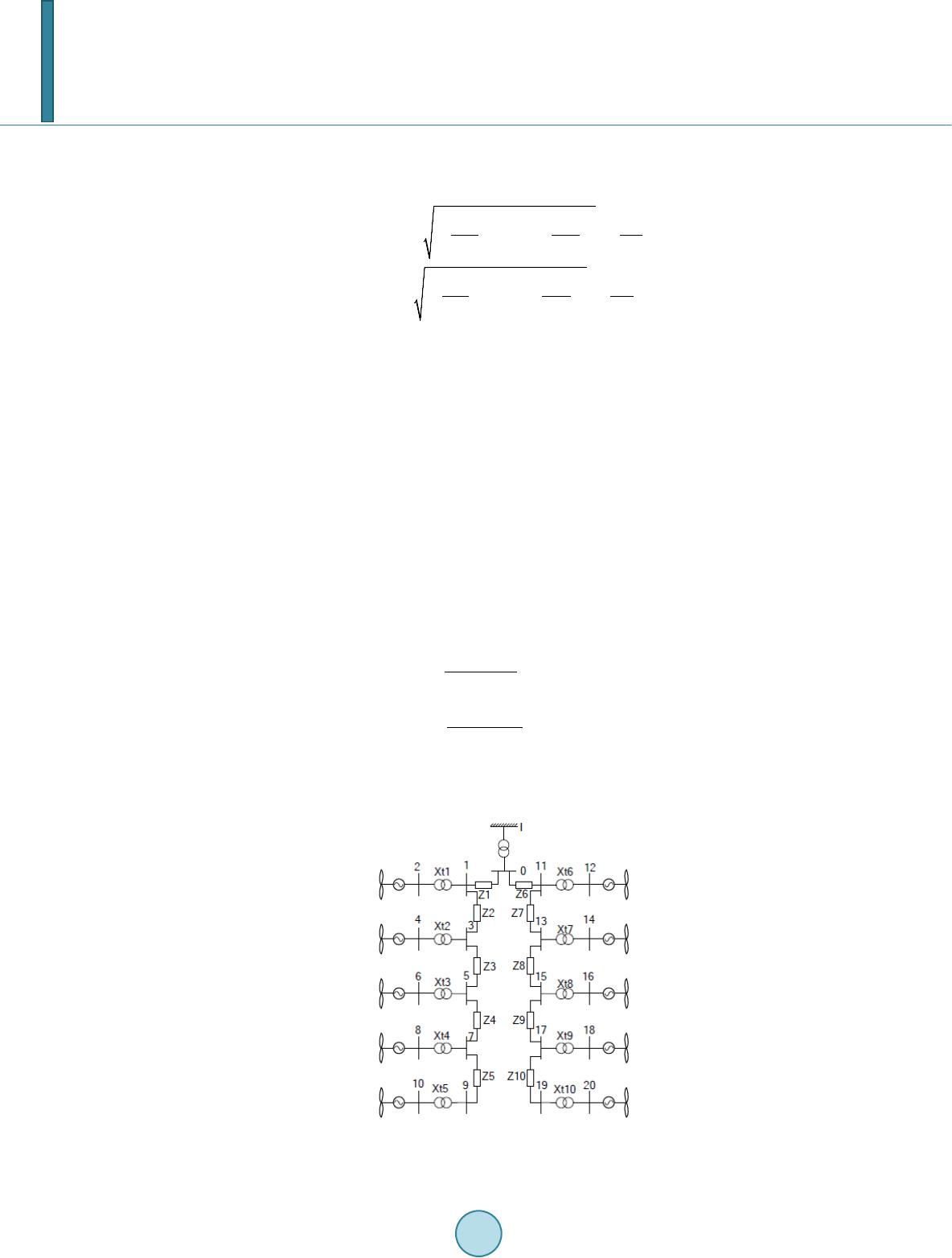 X. Du et al. verter controller is set to 1.0, therefore, the reactive power of the injection system is similar to the stator side reactive power. When stator voltage is constant, operating ranges of active and reactive power are limited by the rotor side converter maximum current. If the active power is a constant value, reactive power output range is 22 2 22 2 33 1 33 1 gi S M giS R SS gi S M giS R SS PU X Q UI X sX PU X Q UI X sX ≥−− − − ≤ −− − (5) where, , , ,S , are the stator voltage , rotor current, magnetizing reactance, stator reactance and slip of DFIG respectively; , gi are the output active power and reactive power of DFIGs. 4) The node voltage constraints is . (6) where, is Per-unit value of the node voltage in wind farm; , are the minimum and maximum limit for node voltage. The voltage constraint range is taken as [0.9, 1.1] in this paper. 4. Calculation Model Verification 4.1. Model Data and Control St rategies A wind farm consisting of 10*1.5 MW DFIGs is used as an example. As it is shown in Figure 3, ten wind tur- bines are divided into two groups, through 10 kV double-circuit line access to 10 kV bus bar of 110 kV step up substation, after step up to 110 kV by a transformer, which is connected with infinite power grid [7]. Strategy 1: Distribute power in the traditional way, according to the proportion of the wind power capacity output of each unit, are shown as follows ,max __ ,max 1 ,max __ ,max 1 gi refifarm ref n gi i gi refifarm ref n gi i P PP P Q QQ Q = = = = ∑ ∑ (7) where, , are prediction maximum powers of DFIG; , are dispatching co m- mands for wind farm; , are power instructions assigned to each turbine. Figure 3. Schematic of a wind farm with 10 turbines.  X. Du et al. Strategy 2: Using optimal control strategy, set , , , which means it only takes mi- nimizing active and reactive power deviation in power output and scheduling requirements as objective function, regardless of active power loss. Strategy 3: Using optimal control strategy, set , , , which means it not only takes minimizing active and reactive power deviation in power output and scheduling requirements as objective func- tion, but also takes active power loss into consideration. If wind speed forecasting curve is known, the maximum power of each wind turbine can be captured accord- ing to the wind turbines power curve. Assuming that the maximum power capture for 10 wind turbines of this period are as shown in Table 1. 4.2. Calculation Results The output distribution units of each DFIG under different control strategies are given in Tables 2 and 3 when scheduling request is large as 5 MW/2 MVar and small as 3 MW/1 MVar respectively. As it can be seen from Tables 2 and 3, traditional strategy 1 is only distributes power due to prediction power capacity, but in fact the output power can’t meet the dispatching requirement. In Table 2, according to strategy 1, the power command is 5 MW, while the total output is 4.71 MW because there is 0.29 MW power loss. So strategy 1 can’t satisfy scheduling demand and power loss is large. Both strategy 2 and strategy 3 can satisfy the active and reactive power of scheduling demand. Compared strategy 2 with strategy 3, when the active power loss is to be considered, the active power loss within the wind farm is less and the operation of the wind farm is more efficient. From distribution sets of strategy 3, it can be seen that active and reactive power output of units close to con- nection node are larger, such as node unit 2, 4, 12, 14 in Table 2 whose active power output have reached their maximum output, however, power output of units far from connection node are smaller, such as node unit 10, Table 1. Maximum power available in each turbine. Turbine number 2 4 6 8 10 Total Maximum power 0.65 0.57 0.71 0.68 0.64 Turbine number 12 14 16 18 20 6.36 Maximum power 0.55 0.55 0.71 0.59 0.71 Table 2. Power dispatch of each turbine (5 MW/2 MVar). Turbine number Strategy 1 Strategy 2 Strategy 3 P1 Q1 P2 Q2 P3 Q3 2 0.50 0.20 0.56 0.28 0.68 0.35 4 0.49 0.22 0.55 0.31 0.65 0.31 6 0.52 0.19 0.55 0.26 0.55 0.25 8 0.42 0.18 0.53 0.35 0.46 0.23 10 0.46 0.19 0.52 0.21 0.40 0.18 12 0.47 0.22 0.55 0.31 0.65 0.37 14 0.43 0.23 0.53 0.36 0.62 0.35 16 0.51 0.19 0.55 0.26 0.52 0.20 18 0.54 0.20 0.54 0.21 0.40 0.19 20 0.66 0.18 0.54 0.21 0.40 0.15 Sum 5.00 2.00 5.42 2.76 5.33 2.58 Total power output of wind farm 4.50 1.39 5.00 2.00 5.00 2.00 Power loss 0.50 0.61 0.42 0.76 0.33 0.58  X. Du et al. Table 3. Power dispatch of each turbine (3 MW/1 MVar). Turbine number Strategy 1 Strategy 2 Strategy 3 P1 Q1 P2 Q2 P3 Q3 2 0.30 0.10 0.31 0.15 0.34 0.20 4 0.29 0.11 0.31 0.12 0.23 0.16 6 0.31 0.09 0.31 0.10 0.15 0.16 8 0.25 0.09 0.30 0.12 0.15 0.09 10 0.28 0.10 0.30 0.09 0.15 0.01 12 0.28 0.11 0.31 0.14 0.34 0.21 14 0.26 0.11 0.30 0.12 0.23 0.17 16 0.31 0.09 0.31 0.10 0.15 0.10 18 0.32 0.11 0.30 0.09 0.15 0.00 20 0.40 0.09 0.30 0.09 0.15 0.00 Sum 3.00 1.00 3.05 1.12 3.04 1.10 Total power output of wind farm 2.80 0.89 3.00 1.00 3.00 1.00 Power loss 0.20 0.11 0.05 0.12 0.04 0.10 20. The reason is that electrical distance of units close to connection node are shorter and their power loss are lower while electrical distance of those far away are longer and power loss are larger. As a result, the unit which is closer should provide more power output to grid in order to meet the objective function that minimizes the power loss within wind farm. 5. Conclusions In this paper, a global optimization strategy is developed for active and reactive power dispatch in a wind farm. This strategy allows following wind farm dispatch center requests, regarding active/reactive power to be gener- ated. The approach was tested with a small wind farm having 10 generators and with different wind power availability scenarios and generation requests. The results proved the effectiveness of the developed approach, demonstrating its practical value in cases where wind farm are requested to follow specific time sequence gen- eration profiles. The proposed approach is flexible enough to be used for different operational strategies. In the dispatch problem, the capability curves of DFIGs of the wind park and circuit line power loss are taken into ac- count. The re-design analysis illustrates that increase in income of 5-10% is possible if the operational strategy is op- timized with respect to both wind conditions and electricity market spot price. Acknowledgements This work was supported by “the Fundamental Research Funds for the Central Universities of China”. References [1] Le, H.T. and Santoso, S. (2007) Analysis of Voltage Stability and Optimal Wind Power Penetration Limits for a Non- Radial Network with an Energy Storage System. IEEE Power Engineering Society General Meeting, Tampa, 24-28 June 2007, 1-8. [2] Jauch, C., Sørensen, P. and Bak-Jensen, B. (2004) International Review of Grid Connection Requirements for Wind Turbines. Nordic Wind Power Conference, Chalmers University of Technology. [3] Pena, R., Clare, J.C. and Asher, G.M. (1996) Doubly Fed Induction Generator Using Back-to-Back PWM Converters and Its Application to Variable-Speed Wind Energy Generation. IEE Proceedings of Electric Power Applications, 143, 231-241. [4] Ekanay ake, J. Holdsworth, L. and Jenkins, N. (2003) Control of DFIG wind turbines. Power Engineer Journal, 17, 28-  X. Du et al. 32. http://dx.doi.org/10.1049/pe:20030107 [5] Hansen, A.D., Sørensen, P., Iov, F. and Blaabjerg, F. (2006) Centralized Power Control of Wind Farm with Doubly Fed Induction Generators. Renewable Energy, 3, 936-951. [6] Zhao, B., Wang, M.-Y., Li, H. and Yang, C. (2012) Optimal Power Dispatch and Control of Wind Farm Based on Nonlinear Interior Point Algorithm. Power System Protection and Control, 40, 24-30. [7] Moya no, C.F. and Lopes, J.A.P. (2007) An Optimization Approach for Wind Turbine Commitment and Dispatch in a Wind Park. Electric Power Systems Research, 79, 71-79.
|