Journal of Power and Energy Engineering, 2014, 2, 176-185
Published Online April 2014 in SciRes. http://www.scirp.org/journal/jpee
http://dx.doi.org/10.4236/jpee.2014.24025
How to cite this paper: Ren, Y. and Suganthan, P.N. (2014) Empirical Mode Decomposition-k Nearest Neighbor Models for
Wind Speed Forecasting. Journal of Power and Energy Engineering, 2, 176-185. http://dx.doi.org/10.4236/jpee.2014.24025
Empirical Mode Decomposition-k Nearest
Neighbor Models for Wind Speed
Forecasting
Ye Ren, P. N. Suganthan
School of Electrical and Electronic Engineering, Nanyang Technological University, Singapore City, Singapore
Received December 2013
Abstract
Hybrid model is a popular forecasting model in renewable energy related forecasting applications.
Wind speed forecasting, as a common application, requires fast and accurate forecasting models.
This paper introduces an Empirical Mode Decomposition (EMD) followed by a k Nearest Neighbor
(kNN) hybrid model for wind speed forecasting. Two configurations of EMD-kNN are discussed in
details: an EMD-kNN-P that applies kNN on each decomposed intrinsic mode function (IMF) and
residue for separate modelling and forecasting followed by summation and an EMD-kNN-M that
forms a feature vector set from all IMFs and residue followed by a single kNN modelling and fore-
casting. These two configurations are compared with the persistent model and the conventional
kNN model on a wind speed time series dataset from Singapore. The results show that the two
EMD-kNN hybrid models have good performance for longer term forecasting and EMD-kNN-M has
better performance than EMD-kNN-P for shorter term forecasting.
Keywords
Wind Speed Forecasting; Empirical Mode Decomposition; k Nearest Neighbor
1. Introduction
Wind energy generated by wind turbines is a potential renewable energy for fossil energy complementary.
However, wind energy is intermittent thus more difficult to be integrated to the grid than power generated by
conventional generators. In order to utilize the wind energy, accurate forecasting is necessary so that the distri-
bution grid has a controllable demand-supply equilibrium [1].
The empirical relation between wind speed and wind power follows a non-linear function (3rd order) and so it
prefers forecasting wind power generated by the wind turbine to the wind speed due to less accumulated error.
However, wind speed data is usually easier to obtain even without the presence of the wind turbine, thus this
paper will focus on wind speed forecasting.
Wind speed time series (TS) is a one-dimensional vector that each value in the vector consists of a wind speed
value and a time-stamp. Some statistical models such as Autoregressive Moving Average (ARMA) can be used
for TS modelling and forecasting and was employed for wind speed/power TS forecasting [2]. However, ARMA

Y. Ren, P. N. Suganthan
177
is a linear model but the nonlinear wind speed TS is not suitable for linear modelling. Some Computational In-
telligence (CI) based models were applied for wind speed/power TS forecasting [3], [4]. These CI based models
were evaluated and compared with statistical models and the results showed that they usually outperform statis-
tical models.
Hybrid models are developed by combining more than one model together. There are mainly four kinds of
hybridization: (i) a linear forecasting model followed by a non-linear forecasting model such as ARMA-Neural
Network (NN) [5]; (ii) an optimization tool to find the optimal parameters for the forecasting model such as
Genetic Algorithm (GA)/Partial Swarm optimization (PSO)-Support Vector Regression (SVR) [6]; (iii) a de-
composition tool to decompose the TS into several sub-TS and different forecasting models to different sub-TS
such as Wavelet-SVR [7] and Empirical Mode Decomposition (EMD)- NN [8] and (iv) a further combination of
the previous three kinds such as Wavelet-PSO-Adaptive Neuro-Fuzzy Inference System (ANFIS) [9].
EMD is a non-linear and non-stationary TS decomposition tool [10]. It decomposes a TS into a collection of
Intrinsic Mode Functions (IMFs) and one Residue. Each IMF or Residue reflects a certain characteristic of the
original TS, which is less complex than the original TS. The details of EMD are described in Section II-A.
In the literature, there are several hybrid models consisting EMD and statistical/CI based models such as
EMD-SVR [11], EMD-NN [8] and EMD-MA-Persistent [12]. However, there are simpler models consisting
EMD and k-Nearest Neighbor (kNN) for TS forecasting. The advantage if kNN is that it is simple, non-parame-
tric and robust.
In [13], an EMD-kNN model was reported for annual average rainfall forecasting. The EMD-kNN model was
used to forecast two rainfall datasets in China and the performance was evaluated by three error measures. The
results showed that the EMD-kNN model outperformed kNN model with respect to all three error measures for
the two datasets. EMD-kNN model was also employed for financial TS forecasting [14]. Four stock TS were
used for evaluation against kNN and ARMA models and the EMD-kNN model was the most accurate one.
This paper applies two configurations of EMD-kNN models for wind speed forecasting: one is to construct
feature vectors for each IMF or Residue and the other is to construct a feature vector set from all IMFs and Re-
sidue. The detailed configurations of the two EMD-kNN models are discussed in Section III.
The remaining of the article is organized as follows: Section II introduces EMD and kNN. Section III dis-
cusses the two configurations of EMD-kNN models. Section IV evaluates the two models with a wind speed TS
collected in Singapore and Section V concludes the paper and recommends for future work.
2. Methodology
In this section, EMD and kNN are introduced in details.
2.1. Empirical Mode Decomposition
EMD [10] decomposes non-linear and non-stationary complex TS into a finite number of TS known as IMFs
and one residue. The IMF has a well behaved Hilbert transformation so that the instantaneous frequency of the
IMF can be calculated and therefore it is able to locate any event on time and frequency domain with IMF [10].
The procedure of EMD (known as sifting) is as follows [10], [15]:
1) Identify all local maxima and local minima in the TS
x(t)
and interpolate all local maxima with an inter-
polationmethod such as cubic spline to form an upperenvelope
max
e (t)
and use the similar interpolationmethod
for all local minima to form a lower envelope
min
e (t)
.
2) Calculate the mean of upper and lower envelopes
( )
max min
ete (t)
m(t) 2
+
=
3) Subtract m(t)from the original TS to obtain a detail component
d(t)x(t) m(t)= −
.
4) Iterate on
d(t )
for the previous three steps until the stopping criteria met.
5) Iterate on
m(t)
for the previous four steps for another IMF formation.
The stopping criteria defined in [10] are: (i) in the whole TS, the number of zero-crossings and the number of
extremamust equal or differ at most by one; and (ii) the mean value of the envelope must approach zero.
However, it is difficult to implement the two above criteria in computing and therefore an additional quantita-
tive criterion is defined by Rilling [15]:

Y. Ren, P. N. Suganthan
178
Define a mode amplitude
( )( )
max min
ete(t)
at 2
−
=
, and define an evaluation function
( )( )
( )
mt
δtat =
. The
sifting iteration stops when
()
1
δtθ <
for
(1 α)−
fraction of the total duration and
2
δ(t) θ<
for
α
fraction
of the total duration.
Where
12
θ,θ
and
α
are user-defined thresholds.
Finally, the original TS is decomposed as:
( )
N
iN
i1
x tIMFR
=
= +
∑
(1)
2.2. k Nearest Neighbor
kNN is a method developed for both classification and regression. It is a kind of lazy learning [16]. The advan-
tage of kNN is that it is a non-parametric model and therefore it can be applied to wide range of applications
[13].
The procedure of kNN for regression is as follows [13], [17]:
1) Form
d
-dimensional feature vectors Dfrom the historicaldata
x
:
t t1td1
D{x ,x,,x}
− −+
= …
; Their corres-
ponding successors are denoted as
h
x
.
2) Form a
n
-dimensional distance vector
i
DIST
foreach testing vector
i
D
by calculating the Euclidean
distance between
i
D
and the remaining
D
:
i ij
DIST{|| DD||}, ji.=−≠
3) Sort
i
DIST
in ascending order and select the first
K
entries as the nearest neighbors
k
D,k{1,. . .,K}∈
.
4) Form a kernel function
( )
K
j1
1/ j
Kj 1/ j
=
=∑
as a weighted averaging factor for kNN aggregation.
5) Calculate the final estimation as
( )
k
hh
j
j1
ˆ
xK jx
=
=
∑
．Where
j
x
is the corresponding successors of
j
D
.
In order to have a better generalization, kNN undergoes a leave-one-out cross validation during training to
select the optimal kand d [17].
3. Two EMD-kNN Models
In the previous section, the details of EMD and kNN are discussed. The advantage of kNN as a regression tools
is also discussed. However, when the TS is non-stationary and nonlinear, there will be difficulties in feature
vector formation, weighted aggregation and so on [13]. A hybrid model consisting EMD and kNN is then intro-
duced to overcome the drawbacks of kNN.
This section discussed two configurations of EMD-kNN: (i) kNN modelling for each IMF and Residue and (ii)
kNN modelling by constructing feature vectors from all IMFs and Residue. We denote the first configuration as
EMD-kNN-Parallel (EMD-kNN-P) and the second configuration as EMD-kNN-Multiple-Features (EMD-kNN-
M). The flowchart of the two configurations is shown in Figure 1. The details of the two configurations are dis-
cussed in the following subsections.
3.1. EMD-kNN-P
EMD-kNN-P applies kNN to each IMF and Residue. The mathematical representation is shown:
h
iii ii
ˆ ˆ
yxkNN(IMF , K,d)= =
(1)
h
R RRR
ˆ ˆ
yxkNN(R,K ,d ) = =
)2(
N
hiR
i
ˆ ˆˆˆ
yxy y= =+
∑
)3(
where
kNN(x,k,d)
is a conventional kNN process described in Section II-B.
The advantage of EMD-kNN-P is that we can use leave-one-out cross validation to select the optimal k and

Y. Ren, P. N. Suganthan
179
Figure 1. Flow chart of the two EMD-kNN models: (a) EMD-
kNN-P and (b) EMD-kNN-M.
d for each IMF and Residue series but the disadvantage is that it requires more computing power as there are
Ntimes more kNN executed for EMD-kNN-P than the conventional kNN.
3.2. EMD-kNN-M
EMD-kNN-M forms the feature vector by combining decomposed historical data. It is advantageous over the
conventional kNN that the EMD-kNN-M’s feature vector contains more information and thus the distance
measure is more resistance to non-linearity and non-stationarity. The mathematical representation is shown:
{ } ( )
hi
ˆ ˆ
yxkNNIMF,R,k,d ,i{1,,N}= =∈…
(5)
Compared with EMD-kNN-P, there are less kNN processes in EMD-kNN-M. Compared with the convention-
al kNN, there is more information in the feature vectors.
4. Results and Discussion
The wind speed was recorded by an anemometer on top of an apartment building located at 78 Marine Dr., Sin-
gapore. The data was collected from May to Jun 2013 with 10 minute average. The dataset was split into five
weekly datasets (WK17 to WK21) for evaluation. The beginning 70% was used for training and the remaining
30% was used for testing. The 5 datasets were scaled to [0,1] interval. An example of the EMD decomposed TS
for WK17 training set is shown in Figure 2.
To evaluate the performance of the models, three error measures are used in the experiment: Root Mean
Square Error (RMSE), symmetric Mean Absolute Percentage Error (sMAPE) and Mean Absolute Scaled Error
(MASE):
( )
2
ˆ
RMSEE[ yy]= −
(6)
ˆ
yy
sMAPE E100%
ˆ
yy
−
= ×

+

)7(
n
jj
j1
n
i i1
i
ˆ |yy |
MASE n|yy |
n1
=
−
−
=
−
−
∑
∑
)8(
where
ˆ
y
is the predicted data,
y
is the desired data and
n
is the number of data points in the TS.
As shown in Table 1, the error measures had an increasing trend with respect to forecasting horizons for the
persistent model but the trend is not consistent increasing for kNN, EMD-kNN-P or EMD-kNN-M. The RMSE,

Y. Ren, P. N. Suganthan
180
Figure 2. An Example IMFs (first 5 TS) and Residue (last TS) of WK17 Training Set after EMD.
Table 1. Comparison of different models on RMSE, sMAPE and MASE for 1, 3, 5, 7 and 9 steps ahead forecasting.
sMAPE and MASE plots with respect to forecasting horizon for the persistent model, the kNN, the EMD-
kNN-M and the EMD-kNN-P on the five datasets are shown in Figures 3-5.
Compared with the persistent model, kNN, EMD-kNN-P and EMD-kNN-M had higher error measures for 1
and 3 step-ahead forecasting in most of the cases but the error measure of kNN, EMD-kNN-P and EMD-kNN-M
became smaller than the persistent model for 7 and 9 step-ahead forecasting. We can infer that kNN, EMD-
kNN-P and EMD-kNN-M have better performance than the persistent model for longer term forecasting.
kNN had smaller error measures than EMD-kNN-P but larger error measures than EMD-kNN-M for 1, 3 and
5 step-ahead forecasting in most of the cases. For 7 and 9 step-ahead forecasting, kNN had larger error measures
than EMD-kNN-M and EMD-kNN-P.
The error measures for EMD-kNN-M for 1 and 3 step-ahead forecasting were smaller than that for EMD-
kNN-P in most of the cases but the error measures for EMD-kNN-M for 5, 7 and 9 step-ahead forecasting were
larger than that for EMD-kNN-P. Therefore we can conclude that EMD-kNN-P is the best model for longer term
forecasting among the four models. EMD-kNN-M has advantage in shorter term and mid-term forecasting.
5. Conclusion and Future Work
This paper has described two configurations of EMD based kNN models for wind speed forecasting. The first
configuration has applied kNN on each IMF and residue and has aggregated the predicted values to form a final

Y. Ren, P. N. Suganthan
181
Figure 3. RMSE v.s. Horizon Plots for WK17, WK18, WK19, WK20 and WK21 datasets.

Y. Ren, P. N. Suganthan
182
Figure 4. sMAPEv.s. Horizon Plots for WK17, WK18, WK19, WK20 and WK21 datasets.

Y. Ren, P. N. Suganthan
183
Figure 5. MASE v.s. Horizon Plots for WK17, WK18, WK19, WK20 and WK21 datasets.

Y. Ren, P. N. Suganthan
184
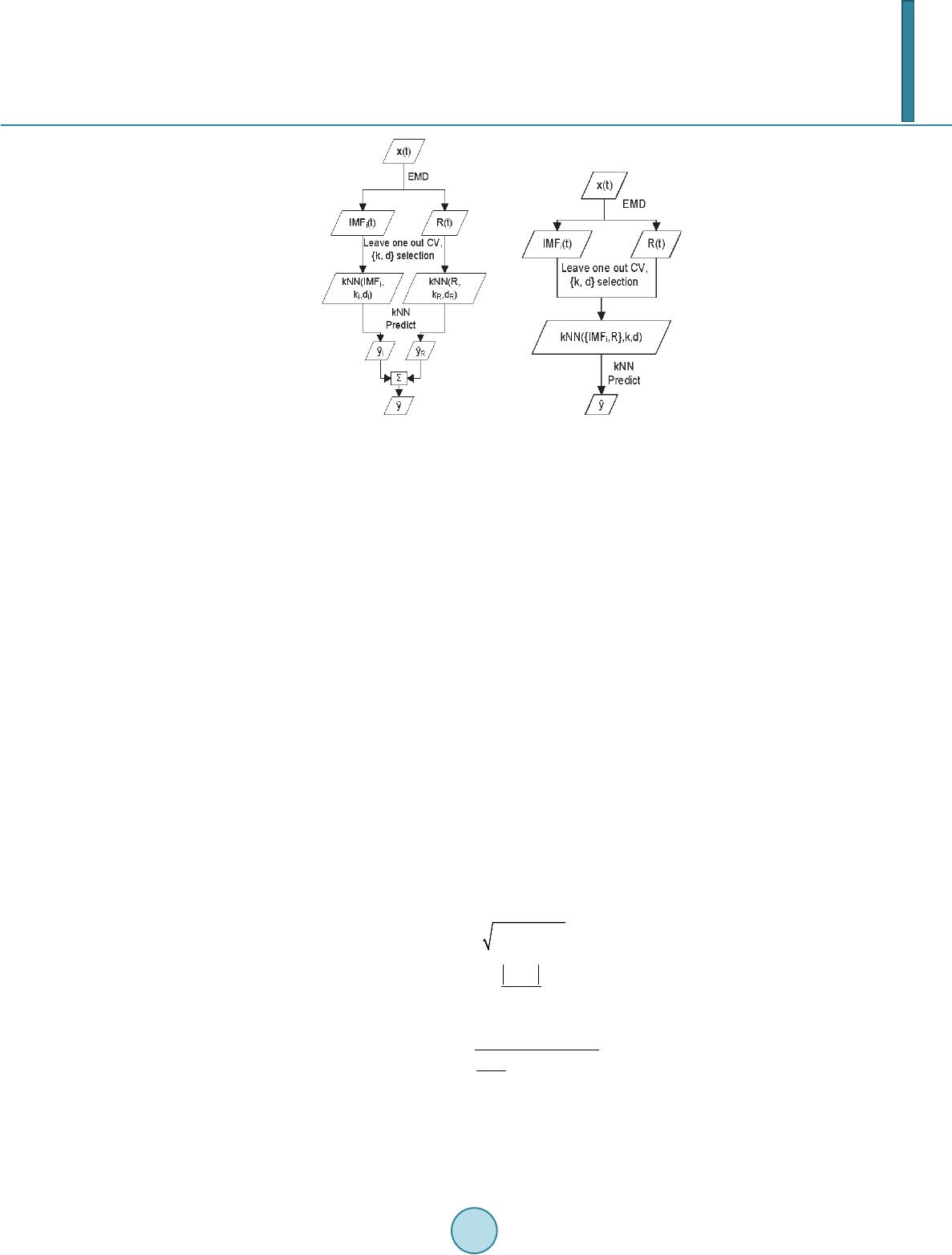
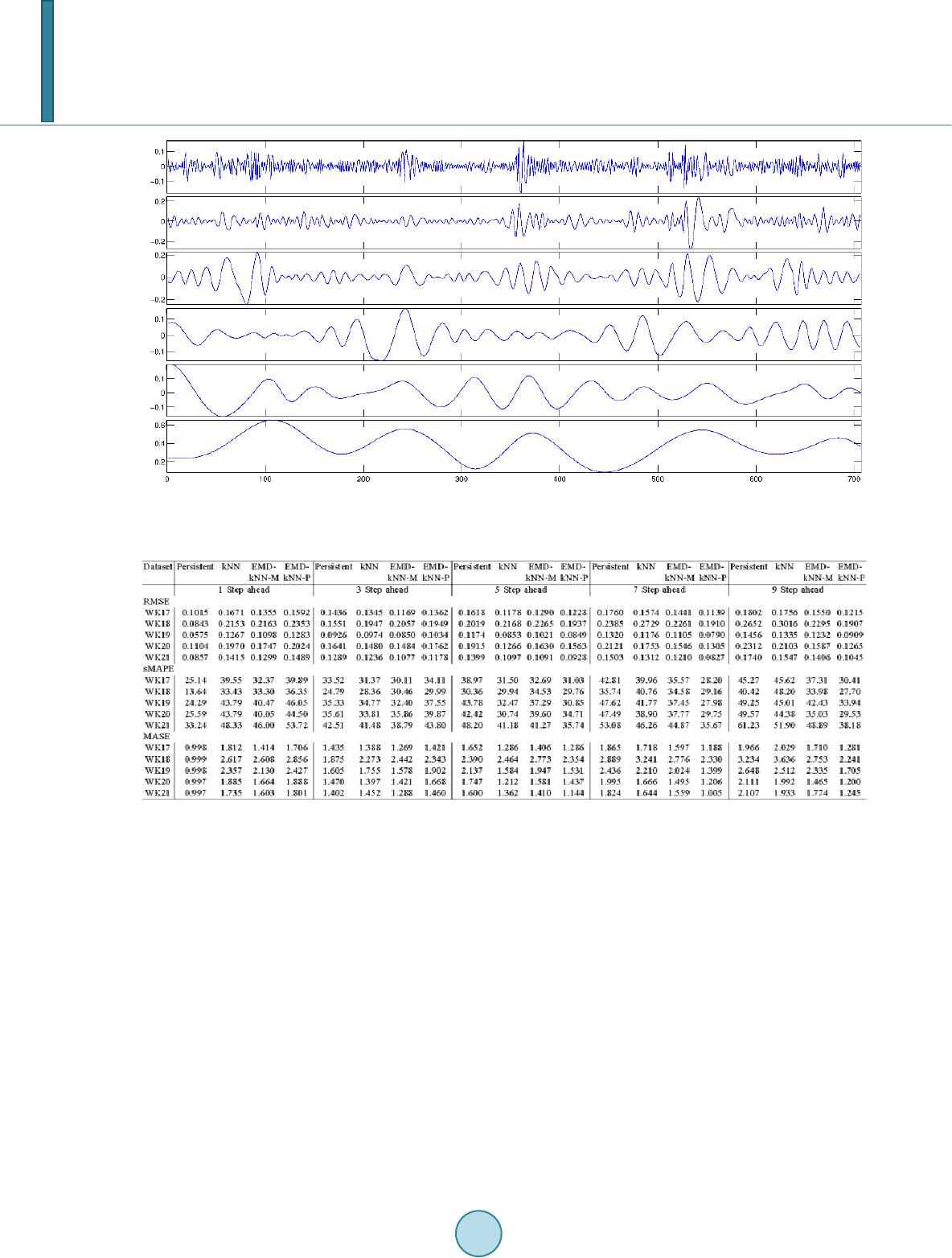
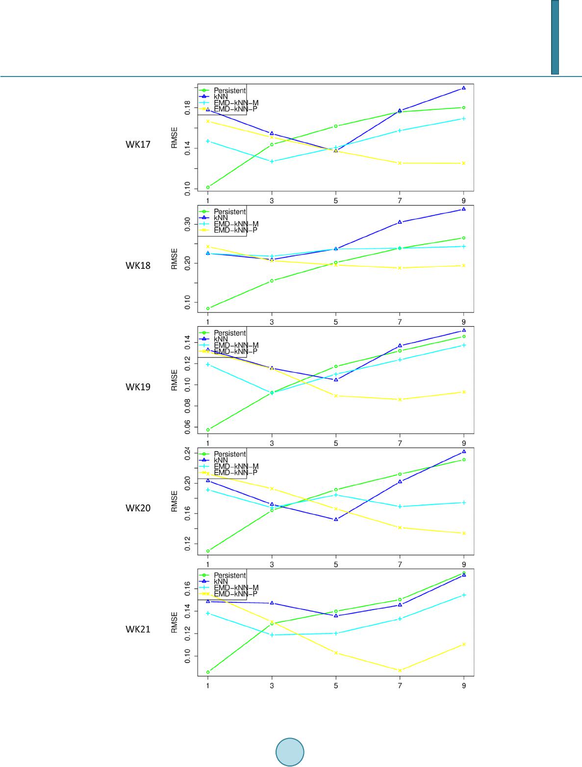
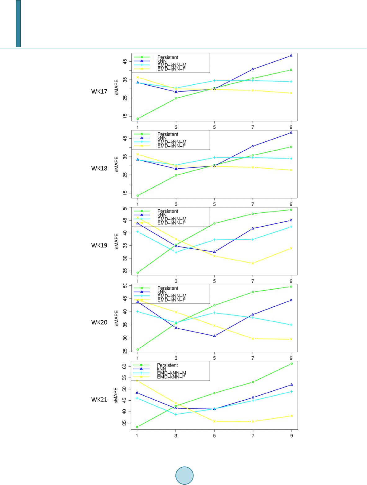
prediction. The second configuration has combined all IMFs and residue together to form a feature vector set for
computing the distance matrix and the prediction has followed the conventional kNN model. The two configura-
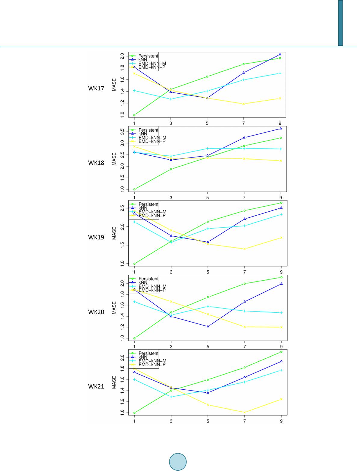
tions have been compared with the persistent model and the kNN model with a wind speed TS recorded in Sin-
gapore. The results have shown that the two configurations outperformed the persistent model and kNN for
longer term forecasting. The second configuration has outperformed the first configuration for 1 and 3 step-
ahead forecasting.
For future work, a possible improvement is on the feature vector selection. Some statistical methods can be
applied for the dimension selection instead of user-defined range followed by grid search based on cross valida-
tion performances. Another possible future work is to apply different weight scheme w to the distance matrix
creation stage. Instead of a uniform w, a linear or exponential decayed w can be used to weigh the distance. This
weighted distance may improve the selection of nearest neighbors.
Acknowledgements
The author Ren Ye would like to thank National Research Foundation (NRF) for providing the Clean Energy
Program (CEPO) research scholarship.
References
[1] Wu, Y.K. and Hong, J.S. (2007) A Literature Review of Wind Forecasting Technology in the World. IEEE Lausanne
Power Tech, Lausanne, 1-5 July 2007, 504-509.
[2] Hill, D.C. , McMillan, D., Bel l, K.R.W. and Infield, D. (2012) Application of Auto-Regressive Models to U.K. Wind
Speed Data for Power System Impact Studies. IEEE Transactions on Sustainable Energy, 3, 134-141.
http://dx.doi.org/10.1109/TSTE.2011.2163324
[3] Damousis, I., Alexiadis, M., Theocharis, J. and Dokopoulos P., (2004) A Fuzzy Model for Wind Speed Prediction and
Power Generation in Wind Parks Using Spatial Correlation. IEEE Transactions on Energy Conversion, 19, 352-361.
http://dx.doi.org/10.1109/TEC.2003.821865
[4] Salcedo-Sanz, S., Ortiz -Garcia, E.G., Perez-Bellido, A.M., Portilla-Figueras, A. andPrieto, L. (2011) Short Term Wind
Speed Prediction Based on Evolutionary Support Vector Regression Algorithms. Expert Systems with Applications, 38,
4052-4057. http://dx.doi.org/10.1016/j.eswa.2010.09.067
[5] Shi, J., Guo, J. and Zheng, S. (2012) Evaluation of Hybrid Forecasting Approaches for Wind Speed and Power Genera-
tion Time Series. Renewable and Sustainable Energy Reviews, 16, 3471-3480.
http://dx.doi.org/10.1016/j.rser.2012.02.044
[6] Wang, Y., Niu, D. and Ma, X. (2010) Optimizing of SVM with Hybrid PSO and Genetic Algorithm in Power Load
Forecasting. Journal of Networks, 5, 1192-1200. http://dx.doi.org/10.4304/jnw.5.10.1192-1200
[7] Zeng, J. and Qiao, W. (2012) Short-Term Wind Power Prediction Using a Wavelet Support Vector Machine. IEEE
Transactions on Sustainable Energy, 3, 255-264. http://dx.doi.org/10.1109/TSTE.2011.2180029
[8] Guo, Z., Zhao, W., Lu, H. and Wa ng, J. (2012) Multi-Step Forecasting for Wind Speed Using a Modified EMD-Based
Artificial Neural Network Model. Renewable Energy, Elsevier, 37, 241-249.
http://dx.doi.org/10.1016/j.renene.2011.06.023
[9] Catalao, J., Pousinho, H. and Mendes, V. (2011) Hybrid Wavelet-PSO-ANFIS Approach for Short-Term Wind Power
Forecasting in Portugal. IEEE Transactions on Sustainable Energy, 2, 50-59.
[10] Huang, N., Shen, Z., Long, S., Wu, M., Shih, H. , Zheng, Q., Yen, N., Tung, C. and Liu, H. (1998) The Empirical Mode
Decomposition and Hilbert Spectrum for Nonlinear and Nonstationary Time Series Analysis. Proceedings of the Royal
Society London A, 454, 903-995. http://dx.doi.org/10.1098/rspa.1998.0193
[11] Ye, L. and Liu, P. (2011) Combined Model Based on EMD-SVM for Short-Term Wind Power Prediction. Proceedings
of the CSEE, 31, 102-108.
[12] Sun, C., Yuan, Y. andLi, Q. (2012) A New Method for Wind Speed Forecasting Based on Empirical Mode Decompo-
sition and Improved Persistence Approach. Conference on Power & Energy (IPEC2012), Ho ChiMinh City, 659-664.
[13] Hu, J., Wang, J. and Zeng, G. (2013) A Hybrid Forecasting Approach Applied to Wind Speed Time Series. Renewable
Energy, Elsevier, 60, 185-194. http://dx.doi.org/10.1016/j.renene.2013.05.012
[14] Lin, A.J. , Shang, P.J. , Fen g, G. C. and Zhong, B. (2012) Application of Empirical Mode Decomposition Combined with
K-Nearest Neighbors Approach in Financial Time Series Forecas ting. Fluctuation and Noise Letters, 11.
http://dx.doi.org/10.1142/S0219477512500186

Y. Ren, P. N. Suganthan
185
[15] Rilling, G., Flandrin, P. and Goncalves, P. (2003) On Empirical Mode Decomposition and Its Algorithms. IEEE -
EURASIP Workshop on Nonlinear Signal and Image Processing (NSIP2003), 3, 8-11.
[16] Solomatine, D.P., Ma s ke y , M. andShrestha, D. L. (2008) Instance-Based Learning Compared to Other Data-Driven
Methods in Hydrological Forecasting. Hydrological Processes, 22, 275-287. http://dx.doi.org/10.1002/hyp.6592
[17] Lall, U. and Sharma, A. (1996) A Nearest Neighbor Bootstrap for Resampling Hydrologic Time Series. Water Re-
sources Research, 32, 679-693. http://dx.doi.org/10.1029/95WR02966