 Journal of Modern Physics, 2011, 2, 97-108 doi:10.4236/jmp.2011.23016 Published Online March 2011 (http://www.SciRP.org/journal/jmp) Copyright © 2011 SciRes. JMP Computer Models of Helical Nanostructures Victor F. Pleshakov Scientific-Research Institute of Electrical Carbon Products, Elektrougli, Russia, E-mail: victorpleshakov@list.ru Received October 22, 2010; revised December 24, 2010; accepted December 27, 2010 Abstract A task of mapping a hexagonal grid to different types of helical surfaces including nanocones, nanotubes and nanoscrolls by unfolding a given surface to a carbon layer plane has been solved. Basing on these models, polyhedric models with all atomic bonds being constant and equal to 1.42Ǻ as in a flat carbon layer have been built, and an algorithm of coloring all faces of such models has been developed. Received models can be utilized for visual demonstration of the helical growth of nanotubes, nanocones, nanofiber and other nanoobjects, and also for physical properties calculation. Keywords: Computer Models of Helical Nanostructures 1. Introduction It seems obvious that 3D-images of nanoobjects play significant role in understanding their geometry, struc- ture and properties. Special literature accumulates reach experimental materials obtained with electronic micro- scopes confirming the spiral or helical growth of nano- cones [1], graphite whiskers [2], nanofiber [3-8], nano- tubes [8-10] and so on. Different helical or spiral growth of nanoobjects models are suggested and discussed; these models, however, are merely sketchy. That’s why a need to develop computer models and general algorithms of building them has arisen. Such algorithms should exflat or at least imitate the growth mechanisms of nanoobjects. The necessity for such models often appears during de- coding of a nanomaterial structure with x-ray, electronic microscope and other methods. The current notion of nanofibers as objects with cones inserted into each other doesn’t exflat experimentally observed cone’s opening angles. As shown in [1,11] there are only five types of nanocones with opening angles δ = 19.19°, 38.94°, 60°, 83.62° and 112.88°, and most of angles observed with electronic microscope do not match these five standard ones; and only in a helicoid the δ angle can vary widely. For instance, [1] adduces opening angle data for dif- ferent carbon fibers between 2.7° and 14.5°, and suggests a helical growth model for nanofibers with open and closed vertex of a cone. In [2], carbon whiskers were produced during the treatment of wood over a SiC cata- lyst. They had the δ angle within 110° - 151°. In [3], car- bon fiber was produced from oil pitch with opening an- gle varying from 60° to 180°. Reference [1] examines a helical growth of nanocones and nonofiber, and [10] examines that of nanotubes. The catalytic synthesis of carbon nanotubes and nanofiber is described in [12], where the question of spiral nanofiber synthesis was also touched. Similar models were used in [4,5] to describe the result of a nanofiber growth over catalysts. Graphite has a flake structure, so it delaminates to separate layers or packs of several layers when it is being exposed to laser evaporation or an arc discharge. Upon loosing stability, layers may roll up to a scroll or conical and cylindrical helixes. Reference [13] suggests a mechanism of dislocational forming of single-shell or multi-shell nanotubes from that scroll, and a correspond- ing disclination mechanism for nanocones. These and other multiple experimental data have lead scientists to the idea of a helical or spiral growth of nanoobjects. In recent days [14-16] helical nanostructures, nano- helixes and nanotubes attract the attention of many re- searchers as a possible perspective material to create terahertz generators still not mastered for now. In aforementioned documents, as was stated above, nanoobject models are sketchy, so it is worthwhile to obtain computer models of surfaces with a carbon nano- grid mapped onto them, explaining, at least in a qualita- tive sense, numerous experimental data. Atomic coordi- nates and parameters of a model could be used then to calculate physical characteristics of nanomaterials and to decode their structure.  V. F. PLESHAKOV 98 The purpose of this document is to obtain a general method of mapping a hexagonal carbon grid (Figure 1) to different types of helical surfaces by unfolding the given surface to a carbon layer plane. These ideas and differential geometry methods often used in material cutting [17] and Modeling of Tent Fab- ric Structures [18] have not been used to build complex nanoobject models, such as helical, as far as we’re con- cerned. Explicitly or implicitly they were used for simple surfaces only, such as cylindrical, conical and scrolls [11] that can always be unfolded to a plane. 2. Problem Definition A graphite layer being rolled up to a tube, a roll or a helicoid along the crystallographic direction v = [v1,v2] (Figure 1), where v1, v2 are integer coprime numbers, requires all atomic bonds to be constant. This means the equation system should be solved to build a model in the general case: 22 2 0 ()()( ) ijiji jr 2 ,1,2,,ij n ,, where r0 is the closest spacing between atoms, n – the number of atoms in the model. This system, however, is undefined, and has multiple solutions, so the problem of determining atomic coordi- nates ξ, η, and ζ in the model is solved in two steps. At first, a hexagonal grid is mapped onto the given surface by unfolding it to a plane. Atomic bonds get de- formed and turn to spiral curve segments on that surface. It is known that if the Gauss curvature of a surface is equal to zero, this surface can be unfolded to a plane while keeping lengths and angles between a pair of curves lying on it intact. However such surfaces as heli- cal with the non-zero Gauss curvature can’t be unfolded directly, but they can be split into flat segments so that each one can be unfolded to a plane. This is called a Figure 1. The flat layer atomic coordinate calculation scheme. conditional or an approximate involute. The smaller these segments are, the more accurately a surface is ap- proximated. Unfolding the surface to a carbon layer plane (Figure 1) this way, we get some area, or simply put - a pattern. Atoms captured by this area are reflected on the given surface after “gluing” the pattern back. Such surface is covered by a grid built of equilateral curvilinear hexagons with the side (arc) length equal to the minimal atomic spacing r0 = 1.42. Å The actual atomic spacing measured along the line connecting two adjacent atoms is lesser than r0 and de- pends on the measurement direction. If the radius of a surface curvature strives for infinity, all atomic spacings measured along the line strive to the extreme value r0, like on a plane (Figure 1). For nano- tubes with the diameter D > 6 the error of spacing measurement along the line and along the arc lying on a surface is less than 1%. Å This model is called a curved atomic-bond approxima- tion model, and is a quite good first approximation to the ideal model. With it, elastic, mechanical, electronic and other characteristics of nanotubes are computed, and also hydrogen adsorption and desorption issues are studied. On the second step, atomic coordinates of the model are adjusted so that all atomic bonds would equal to r0 = 1.42 as in a flat graphite layer, and polyhedric models are created basing on the solution of a system of three quadratic equations. Such models were examined in [19,20]. Finally, a not so easy problem of coloring all faces of a polyhedric model is solved. Å Now, let’s take a closer look at these questions. 3. Conical Helicoid Helicoid is a surface produced by rotating a line or a line segment around the chosen axis with the constant angle between the axis and the line equal to δ/2, and by simul- taneous moving that line or a line segment along the axis by bφ value. There are two types of helicoids: a right helicoid (δ = 180º) and an oblique helicoid (δ ≠ 180º). To cover a wider class of surfaces, let’s consider a more complicated version of a helicoid, when a line segment spires along an Archimedean spiral (ρ = aφ) and simultaneously moves along the ζ axis by bφ value. Let’s call this surface a conical helicoid. In particular, having b = 0 we get a conical scroll named by analogy with a cy- lindrical scroll examined in [11]. Figure 2 shows a projection of a conical scroll to the ηζ plane enclosed within two spirals AB and CD, where L is a scroll’s generatrix, δ-opening angle of a cone. The BD segment being rotated around the ζ axis at angle of δ/2 counterclockwise produces conical scroll. If b ≠ 0, a Copyright © 2011 SciRes. JMP  V. F. PLESHAKOV99 scroll unrolls along the ζ axis producing a conical heli- coid described in co-ordinate system having point O as the origin with the following equation: cos ,sin,cos(2),bt (1) where 0sin( 2)t 00 tL, - t- ing radius. star In (1) the σ parameter must not be arbitrary, because the interlayer distance should be constant in a helicoid, or equal to zero in a cone. So let’s present σ as a sum of two items: σ = a + c. The a parameter is responsible for the Archimedean spiral which the BD segment rotates along, while the c parameter keeps the interlayer distance H in a helicoid constant. For t = 0 and t = L the surface enclosed between two spirals (1) is a ruled surface with Gauss curvature equal or not equal to zero, depending on the values of ,,,acb parameters. Coordinates of point (atoms) on the surface of a helicoid must be expressed via coordinates of the flat layer. To map a carbon grid to the given surface we should know how it is unfolded on the plane and find the de- pendence () between the angle ψ on the involute and the angle φ on the surface (1). Let’s study these questions separately. 4. Unfolding Helical Surfaces to a Plane To calculate coordinates of atoms in each model, two coordinate systems are introduced – a moving one with the origin at the О’ point on the Figure 2 and a fixed one with the origin at the О point. Further, we will denote variables ,, and ,, yz in the non-stationary coordinate system with a p index, and in the fixed system – without an index. The Equation (1) is expressed in the non-stationary coordinate system as: sin( 2)cos pR , sin( 2)sin pR , cos( 2) pR (2) One can see, that the expression (2) is an equation of a conical surface with one fixed point О’, where an Archi- medean spiral is a directrix, and the vector R is a genera- trix. Such surface can be unfolded to a plane with both angles and lengths remaining the same. The involute of a surface to the plane xz is a set of spirals covering area : 0 tL cos ,sin, pp xR zR (3) where 0sin( 2)sin( 2)Rt in (2) and (3). To express the equation of a surface and the equation of a spiral on a plane in the stationary coordinate sys- tem one should subtract the value of OO 0cot 2a Figure 2. The projection of a conical scroll to a plane. from z in (3). So we get: , , 0cot 2 pa (4) x 0cot 2 p zz a (5) Now the main problem is to find the dependence we need to map a carbon grid to a surface. Since the arc length of an arbitrary curve on a surface remains invariant while unfolding it to a plane, we can use (2) to get the following equation: 2222222 (dd)dsin2dRRRR 2 , where the left and the right part of the expression are respectively square of arc length of a curve on the plane and on the surface, and denotes derivative on the angle φ. R After several simple transformations we receive the equation ddsin2 1 ; solving it, we find 1sin 2 (6) It seems that such approach can be also used to deter- mine the dependence for undevelopable surfaces, however in this case we will get a more complex equa- tion. The simple way to find the dependence for undevelopable surfaces is as follows. Since an Archi- medean spiral 0sin 2at is a directrix of a conical helicoid (1), we can approximate dd R , where ds – is a length of an arc element of a helix, and sin 2R is an absolute value of a radius-vector drawn from О’ (Figure 2) to that arc element of a helix. Considering the calculation is performed in the stationary coordinate system, we have: 22 1 sin2d = 1 q f , (7) (Figure 2) from in (2) and where Copyright © 2011 SciRes. JMP  V. F. PLESHAKOV Copyright © 2011 SciRes. JMP 100 2 sin 211fqArsh q , 11 ffq , qa (8) If we assume a=0 in the integrand in (7), we auto- matically receive an accurate relation between angles ψ and φ for conical surfaces (6). So we have used (7) to acquire a method of building a conditional (approximate) involute of helical surfaces to a plane, that is, we’ve set a one-one mapping between points (atoms) of the surface and the plane. The calculations show that the dependence (7) is linear and for conical surfaces is approximated by (6) quite good. Besides, it doesn’t depend on the t parameter so it is acceptable to use it for undevelopable surfaces such as helical surfaces as well. In this document, the equation (6) was used to calculate the dependence for all types of the below surfaces, except the general case (1), which has allowed to significantly re- duce calculation time. Figure 3 shows an example involute of a conical scroll to the plane xz in the non-stationary (at the right) and stationary (at the left) coordinate systems. The invo- lute displays an area enclosed between two spirals (3) or (5), when t = 0 and t = L. It is the area, where atoms of a flat carbon layer must be. One can see that in the non-stationary coordinate system all radius-vectors come from the origin (point О’ at the Figure 3). The conical scroll itself with a carbon grid already mapped to it is depicted at the Figure 5. 5. The Method of Mapping a Carbon Grid to a Surface Finally, let’s study a problem of generating atomic coor- dinates of a conical helicoid using the known depend- ency (6), (7) and (8) between φ and ψ angles. Coordinates at the flat layer xi and zi (i = 1,2, ,n), where n is the number of atoms enclosed within the area between two helixes on the xz plane, are known and can be found by corresponding formulas [11]. 11212 220 sinsin ,zalb albz (9) 11212 220 cos cos al balbx , where 12 ,,aa - parameters of an elementary cell at the flat layer, 12 ,0,1,2,,1,2ll , 00 , z- coordi- nates of a nearest hexagon center. The β and α-β angles can be expressed through the identity period 12 ,A by formulas [11]. Coordinates of two basis atoms ex- pressed in fractions of a carbon layer elementary cell period are 0, 0,13, 23b, if . 12 0 Figure 3. The involute of a conical scroll to a plane in the non-stationary (at the right) and stationary (at the left) coordinate systems. Figure 4. The involute of a conical scroll to a carbon layer plane in two coordinate systems - non-stationary (at the left) and stationary (at the right).  V. F. PLESHAKOV101 Figure 5. A conical helicoid with non-overlapped layers: φ1 = 0, φ2 = 6π, δ = 60°, ρ0 = 2.3, H = 3.356, L = 5.64, b = 1.2, v = [3,1], and a conical scroll with a carbon grid mapped to it: φ1 = 0, φ2 = 4π, δ = 60°, ρ0 = 3, H = 3.356, L = 10.47, b = 0, v = [3,1]. Å Å Determining coordinates 12 ,,xl l and 12 ,,zl l of atoms in a flat carbon layer from (9) with pre-defined integer numbers 12 and ,ll , we can write the follow- ing equation in the non-stationary coordinate system for an absolute value of a radius-vector R drawn from the point O′ to an atom on the plane, and the angle ψ: 22 sin ,, ppp 00 RRRL zRR x z (10) where 00 sin 2R . The main difficulty here is to find angles φi for atoms lying on the helical surface using known angles ψi on the involute by solving equations for all atoms f , где 1 (11) where f is found with (8), if . 0a If , then according to (6), 0a sin 2f and 11 fsin 2 . Since the function arcsin p zR expressed from (10) is ambiguous having its principal values lying within 2π2 , it is impossible to find one-one mapping between angles φ and ψ directly. Besides, the angle ψ at the involute, obviously, should change within 0 . To solve this issue, let us split the interval between angles 1 1 and 22 onto segments of 2 the following way: 21pjj f , , 21 1pk f 1, 2,,jk (12) where 21 2πkceil , obviously, 1 and 221 , and the function rounds the number to the nearest integer. ceil Now, for i-th atom let us find the angle arcsin ii zR and determine which quarter of a flat circle the calculated angle hits by analyzing signs of x and z coordinates. For the first quarter of a circle , 0, 0xz ; 0, 0xz for the second and the third 0, 0xz π and, finally, for the fourth quarter , 00,xz2π . Next, we calculate the angle pj , , where p is found with (12), and by using the function 1, 2,,jk zero we find the corresponding angle in according to (11) if for t = 0. 0a 01 ,,,,,, /Ffzerofib t 2 2 @ ,,psi (13) where the ipsi operator calculates the function F 12 ,,jl l,f , and the search of a root of this function starts from the point 12 2 . The integer numbers 12 ,,ll identify atoms, while identifies an interval number as in (12). If , φ is explicitly de- termined from (6): j 0a sin (14) 2 Next, let us calculate the radius 00 , , and for all atoms analyze if the angle sin 2R 00RRt and the radius belong to intervals: R 1pjpj and , 00 RRRL 22 zRx If both conditions are met simultaneously, atomic co- ordinates at the flat layer x and z are stored in arrays , ixziz , while helical atomic coordinates in the stationary coordinate system are calculated using (4). Atomic coordinates in two coordinate systems on a plane are computed using Formulas (3) and (5). Finally, the number of atoms in a model n is calculated. The variable n initially equal to zero gets increased by one every time. Arrays of angles 1 and needed to draw a flat helical involute and enclosed atoms, and also to map a carbon grid to a surface, are created for each atom using (4). 6. Different Surface Types As was previously stated, depending on the values of and b parameters in (1), one can get different types of helical and conical surfaces. Let’s examine these cases. ,ac 1) General case. In this case the interlayer distance H of a helicoid must be constant and roughly equal to that Copyright © 2011 SciRes. JMP  V. F. PLESHAKOV 102 of turbostratic carbon. To make H constant, the values and c in (1), as it follows from Figure 2, must be equal to: a 2πcos 2aH , tan2cb иac . (15) If 02cosbL 2 , then layers are partially overlapped; if 2cos(2)bL - there’s no over- lapping. If , we receive a conical scroll. 0b At Figure 2, the BD segment being rotated is always located at the surface of a conical scroll (b = 0). The ends of this segment (points B and D) on that surface describe two helixes (4), if t = 0 and t = L. Unfolding a conical scroll turns two helixes (4) into spirals (5) on a plane. It is the area cut from a plane by spirals that is the area, where carbon layer atoms must be. An example involute presented at the Figure 4 shows a conical scroll unfolded to a carbon layer plane. The Figure 5 (at the left) shows a conical helicoid and a coni- cal scroll (b = 0) with a carbon grid mapped to them. Calculated parameters are shown on the same pictures. The obtained surfaces can be a visual demonstration of a nanofiber growth, to some extent. 2) Conical surface (a spiral growth of nanocones). This case doesn’t contain a spiral movement, and the BD segment at the Figure 2 rotates at the constant angle to the ζ axis while staying on the surface of a cone all the time. To make this possible, we should put a = 0 in (15). An arbitrary point at the BD segment will describe a conical helix with the radius 0tan 2b sin 2t on the surface of a cone. To make segments not overlap during rotation, the following condition must be met: 2πcos 2bL . If 2πcos 2bL , then two helixes (Figure 2), de- scribed by ends of the segment on a cone’s surface, join together forming a stripe with the width L. Such helical surface being mapped with a carbon grid may visually imitate a spiral growth of nanocones. As shown in [1,11], the angle δ at a conical surface can’t be arbitrary as it is connected with the angle γ at an involute with the fol- lowing correlation: 2πsin 2 , where =60, 120, 180, 240,300. (16) If the condition is met, carbon layers join seamlessly where the helixes meet. Figure 6 shows a surface imitating a spiral growth of a nanocone with 2πcos 2bL , and a conical helix 2πcos 2bL , having in (1). 0H 3) Nanocon es . If one puts σ = 0 and b = 0 in (1) and limits the angle φ within 02π , the following equation of cone can be written: cos ,sin, cos2 ,t where 0sin2t , 0tL . The correlation between φ and ψ in this case is calcu- lated using (6). Seamless join of a carbon layer on the nanocone’s surface is only possible if the angle δ meets (16). Nano- cones are thoroughly examined in [11] by the author by means of unfolding them to a plane and formulating conditions for a seamless join of a carbon layer. 4) Oblique helicoid. Assuming σ = 0 in (1), one can get an equation: cos ,sin, cos2 ,bt (17) where 0sin2t , . 0tL From (15), assuming σ = a + c =0, one can receive c = –a. Figure 7 illustrates this case. The BD segment being rotated by the angle 2π takes the position, and all its points move along the axis ζ by the value 2πb. Points B and D describe two helical curves that entirely lie on the surface of cylinders with radiuses 0 BD and 0sin 2L . The surface enclosed between these two helical curves is an oblique helicoid. To make interlayer distance H constant, the b parameter must be equal 2πsin 2bH . Calculation of the angle φ is performed using formulas (14). Since the radius ρ doesn't depend on the angle φ, an in- volute of a helix to a plane in the non-stationary coordinate Figure 6. A spiral growth of nanocones (at the left) b = (L/2π)cos(δ/2) = 0.70485, and a conical helix (at the right) b = 1.2 > 0.70485, φ1 = 0, φ2 = 7π, δ = 60°, ρ0 = 2.5, H = 0, L = 5.114, v = [5,1]. Copyright © 2011 SciRes. JMP  V. F. PLESHAKOV103 Figure 7. The oblique helicoid calculation scheme. system is a circle with radius sin 2R , that is: cos ,sin, pp xR zR (18) and the area, where atoms of a flat carbon layer must be, is enclosed between two concentric circles with radiuses 10 sin 2R и. 21 Since the angle ψ can take a value within RLR 0 on a plane, then if 2 , then each consequent circle repeats the previous one, that is, they overlap. To acquire the equation of a helix in the stationary co- ordinate system with the origin in O, unlike in (5), one must subtract the value of 0cot 2OO b from the variable z in (18), finally receiving: x 0a cot2 p zz tan22πcos 2ab H . The atomic coordinate in the stationary coordinate system, unlike in (4), is calculated as follows: 0cot 2 pa , where 22 p Rxz. Figure 8 (at the left) shows the surface (17) with a carbon grid mapped to it. 5) One more case of an oblique helicoid. In this case, while the BD is being rotated, the point B at Figure 7 always stands on the plane and circumscribes a circle with radius ρ, while the point D moves along the ζ axis by the value of bφ, describing a helical curve. After turning by 2π, the segment BD takes the CD’ position. An arbitrary point E lying on the segment BD and dis- tant from the point B by t in the coordinate system O describes a helical curve similar to the previous case. The difference is that t has a variable bottom limit, namely cos 2b From the Equation (17), assuming cos 2tb , one can get the equation of a spiral lying on the plane (described by the point C), namely: cos ,sin , 0 , where, 0tan2b (19) and if tL , we receive a spatial helix described by the point D, that is: cos ,sin , cos2 ,bL (20) where 0sin 2L . The segment CD describes a helical surface, and its ends move along two helixes (19) and (20). Since ρ in (19) takes its values within min 0 , where ρ0 and ρmin – maximal (or starting) and minimal values of the radius ρ, the angle φ should be within 0min 0cotb 2 or, assuming 2πsin2bH , 0min 02πcos 2H . Figure 8 (at the right) illustrates this case. 6) Right helicoid (a spiral growth of carbon layers). Assuming δ = 180º and c = 0 in (1), one can get the fol- lowing equation: cos ,sin,,b (21) where 0at , 2πbH , . 0tL If b = 0, then the Equation (21) is a set of spirals. If a = 0 as well, we receive a set of flat circles repeating them selves many times, depending on the angle φ. If 0πaL2 , the areas between two spirals partially overlap when t = 0 и t = L. If /2πaL - no overlap- ping occurs. If 2πaL , the spirals touch each other and imitate the spiral growth of a flat layer. Finally, if b≠0, all spirals unrolls along the ζ axis producing a spa- tial model that imitates the growth of carbon layers. As a result of the dislocation entering the surface, we receive either a stack (a column) of carbon layers in the form of a cylinder, or a cone, or a ring, or a circle on a plane, depending on the values of 01 ,, Lab . The angle φ is calculated from the known angle ψ at the involute using (13) if 0a , or (14) if a = 0. 7. Cylindrical Helicoid Assuming δ = 0 in (1) we can write the following equa- tions: cos ,sin,bt ,where 0a , . (22) 0tL In this case a line segment with the length L parallel to the ζ axis rotates along Archimedean spiral and simulta- tL. The angle φ is calcu- lated through the angle ψ using the same Formula (14). Copyright © 2011 SciRes. JMP  V. F. PLESHAKOV 104 Figure 8. Two types of oblique helicoids imitating a spiral growth of nanofiber. The left picture has the following parameters: φ1 = 0, φ2 = 7π, δ = 60°, ρ0 = 3, H = 3.356, L = 7.44, v = [5,1]. The right picture has the following parameters: φ1 = 0, φ2 = 4.2π, δ = 40°, ρ0 = 10, ρmin = 3, H = 3.356, L = 6.15, v = [2,1]. Å Å neously moves along the ζ axis by bφ. Segment’s ends describe two helixes with t = 0 и t = L. To unfold the surface between these two helixes, it is sufficient to know the length of Archimedean spiral’s arc s and the variable ζ. Substituting x = s и z = ζ, the surface will be unfolded at the xz plane. Considering that 22 dsd , we get the fol- lowing expression for the length of spiral’s arc: s 0ff , where 222 2 aa Arshaa (23) To keep the interlayer distance H constant the follow- ing condition should be met: a=H/2π. If a = 0 in (22), we receive two helixes entirely lying on the surface of a cylinder. To make areas enclosed between them no overlapping, the inequality must be fulfilled: 2bL . If 2πbL, two helixes touch each other and create a stripe with the width L on cylider’s surface. Now, if 01 2π,kA2 , , where 1, 2,k 12 ,A is the identity period [11] in the crystallographic direction 12 , v s , then car- bon layers join seamlessly where the helixes meet. Such surface with a carbon grid mapped onto it visually dem- onstrates a spiral growth of nanotubes. Since 0 in that case, the involute to the plane xz is a set of line segments having their slope ratio about the x axis equal to 0 b , namely 0 zb x t, , , max 0xs 0tL 00 zbxbx L. To map a carbon grid to a surface, one can use the fact that rolling up a flat layer to a helix turns the coordinate (9) 12 ,,xl l , , 12 ,1,2,3,ll1, 2,,b m to an arc of a helix. So we have: 12 ,,xlls , (24) where s is expressed from (23), or 0 s if a=0. If we calculate an angle φ for all atoms using (24), that is, for all legitimate values of l1, l2 and ν, then atomic coordinates on helicoid’s surface can be found from 12 cos,sin,, ,zll (25) The angle φ here is a function of 12 ,иll identify- ing atoms, that is 12 ,,ll . In particular, with b=0 we obtain a common cylindrical scroll already examined in [11]. Figures 9-10 illustrate these cases. We can take as a hypothesis that when the dislocation enters a surface along the z axis, figures pictured at Figures 9-10 (at the left) turn to a scroll or a nanotube (at the right). Further radial movement of the dislocation in the scroll leads to a multi-shell nanotube generation, if the angle φ is divisi- ble by 2π. Otherwise, there is a part of unfinished layer left on nanotube’s surface, and the growth process con- tinues according to [13]. Having determined φ from (24) or from 12 ,,xl l 0 , if a = 0, and assuming z=ζ, one can get the follow- ing inequities for variables x and z that must be fulfilled simultaneously: 12 ,0.00xxx 1 bzbL , and , where 12 ma s x 2 0,xx. If a = 0 и b = 0, and 0π , the resulting surface is a cylindrical surface (nanotube). The condition for a Copyright © 2011 SciRes. JMP 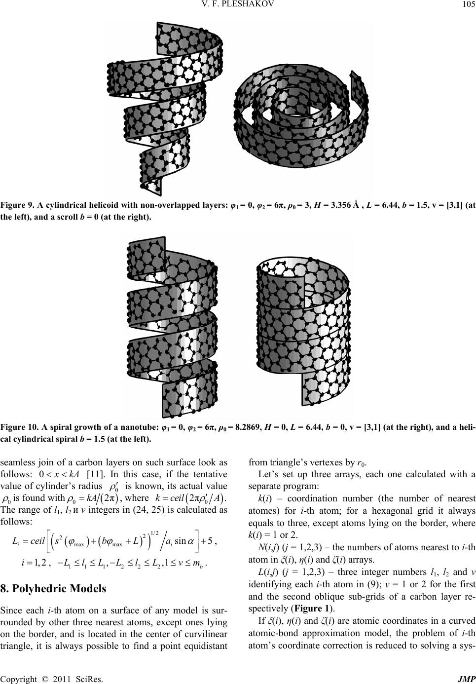 V. F. PLESHAKOV105 Figure 9. A cylindrical helicoid with non-overlapped layers: φ1 = 0, φ2 = 6π, ρ0 = 3, H = 3.356, L = 6.44, b = 1.5, v = [3,1] (at the left), and a scroll b = 0 (at the right). Å Figure 10. A spiral growth of a nanotube: φ1 = 0, φ2 = 6π, ρ0 = 8.2869, H = 0, L = 6.44, b = 0, v = [3,1] (at the right), and a heli- cal cylindrical spiral b = 1.5 (at the left). seamless join of a carbon layers on such surface look as follows: 0 kA [11]. In this case, if the tentative value of cylinder’s radius 0 is known, its actual value 0 is found with 0 2πkA, where 0 2πk ceilA . The range of l1, l2 и ν integers in (24, 25) is calculated as follows: 1/2 2 2 max maxsin 5 i Lceil sbLa i , , . 1, 2i111222 ,,1 b LlLLlLvm 8. Polyhedric Models Since each i-th atom on a surface of any model is sur- rounded by other three nearest atoms, except ones lying on the border, and is located in the center of curvilinear triangle, it is always possible to find a point equidistant from triangle’s vertexes by r0. Let’s set up three arrays, each one calculated with a separate program: k(i) – coordination number (the number of nearest atomes) for i-th atom; for a hexagonal grid it always equals to three, except atoms lying on the border, where k(i) = 1 or 2. N(i,j) (j = 1,2,3) – the numbers of atoms nearest to i-th atom in ξ(i), η(i) and ζ(i) arrays. L(i,j) (j = 1,2,3) – three integer numbers l1, l2 and ν identifying each i-th atom in (9); ν = 1 or 2 for the first and the second oblique sub-grids of a carbon layer re- spectively (Figure 1). If ξ(i), η(i) and ζ(i) are atomic coordinates in a curved atomic-bond approximation model, the problem of i-th atom’s coordinate correction is reduced to solving a sys- Copyright © 2011 SciRes. JMP 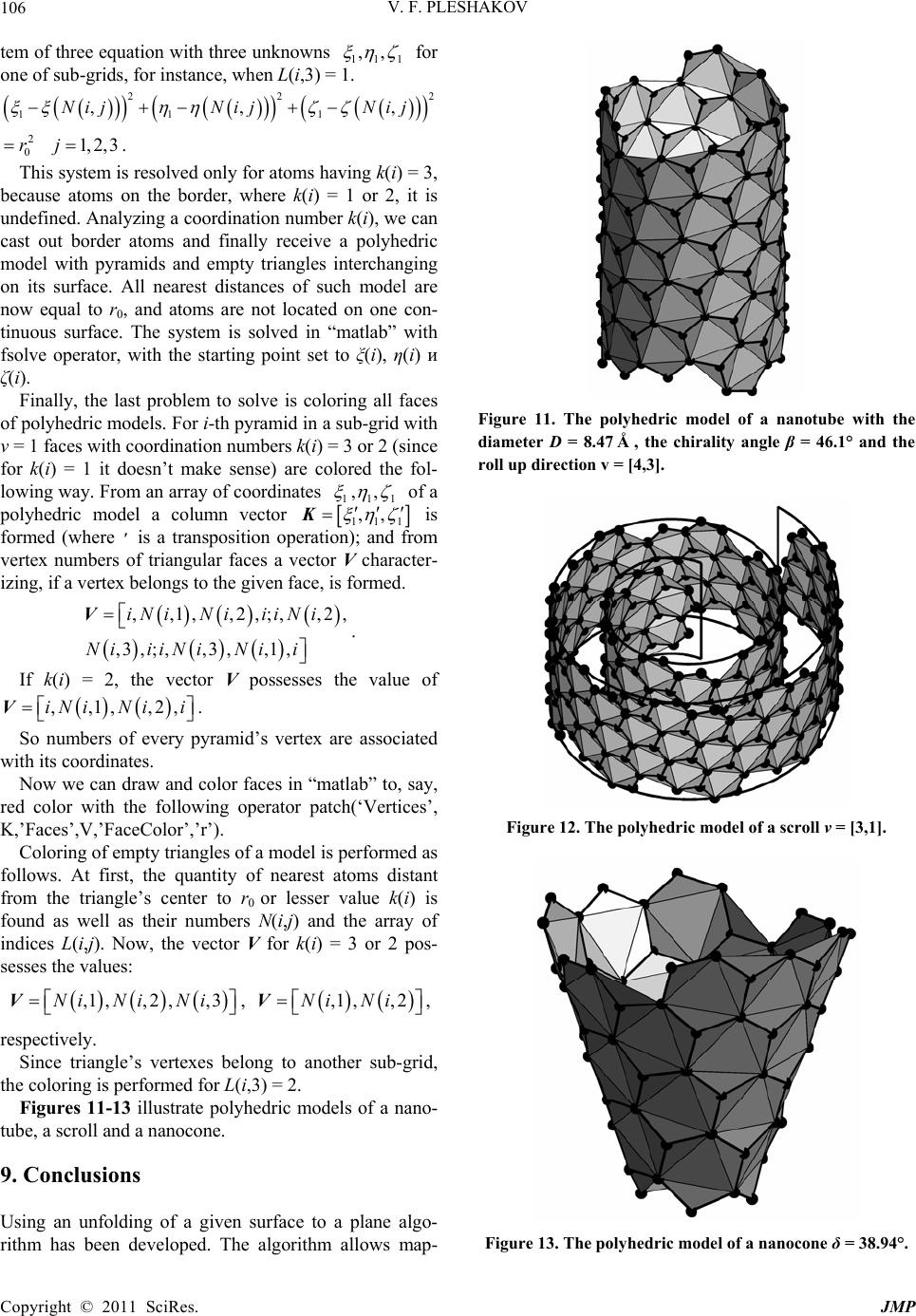 V. F. PLESHAKOV 106 tem of three equation with three unknowns 11 1 ,, for one of sub-grids, for instance, when L(i,3) = 1. 22 111 ,, 2 , ij NijNij 2 0 r . 1,2, 3j This system is resolved only for atoms having k(i) = 3, because atoms on the border, where k(i) = 1 or 2, it is undefined. Analyzing a coordination number k(i), we can cast out border atoms and finally receive a polyhedric model with pyramids and empty triangles interchanging on its surface. All nearest distances of such model are now equal to r0, and atoms are not located on one con- tinuous surface. The system is solved in “matlab” with fsolve operator, with the starting point set to ξ(i), η(i) и ζ(i). Finally, the last problem to solve is coloring all faces of polyhedric models. For i-th pyramid in a sub-grid with ν = 1 faces with coordination numbers k(i) = 3 or 2 (since for k(i) = 1 it doesn’t make sense) are colored the fol- lowing way. From an array of coordinates 111 ,, of a polyhedric model a column vector 11 ,, 1 K is formed (where ׳ is a transposition operation); and from vertex numbers of triangular faces a vector V character- izing, if a vertex belongs to the given face, is formed. ,,1,,2,;,,2 ,3 ,;,,3 ,,1, iN iN iiiN i NiiiNiNi i V, . If k(i) = 2, the vector V possesses the value of . ,,1,,2,iNiN ii V So numbers of every pyramid’s vertex are associated with its coordinates. Now we can draw and color faces in “matlab” to, say, red color with the following operator patch(‘Vertices’, K,’Faces’,V,’FaceColor’,’r’). Coloring of empty triangles of a model is performed as follows. At first, the quantity of nearest atoms distant from the triangle’s center to r0 or lesser value k(i) is found as well as their numbers N(i,j) and the array of indices L(i,j). Now, the vector V for k(i) = 3 or 2 pos- sesses the values: ,1, ,2, ,3Ni NiNi V, ,1 ,,2Ni Ni V, respectively. Since triangle’s vertexes belong to another sub-grid, the coloring is performed for L(i,3) = 2. Figures 11-13 illustrate polyhedric models of a nano- tube, a scroll and a nanocone. 9. Conclusions Using an unfolding of a given surface to a plane algo- rithm has been developed. The algorithm allows map- Figure 11. The polyhedric model of a nanotube with the diameter D = 8.47, the chirality angle β = 46.1° and the roll up direction v = [4,3]. Å Figure 12. The polyhedric model of a scroll v = [3,1]. Figure 13. The polyhedric model of a nanocone δ = 38.94°. Copyright © 2011 SciRes. JMP 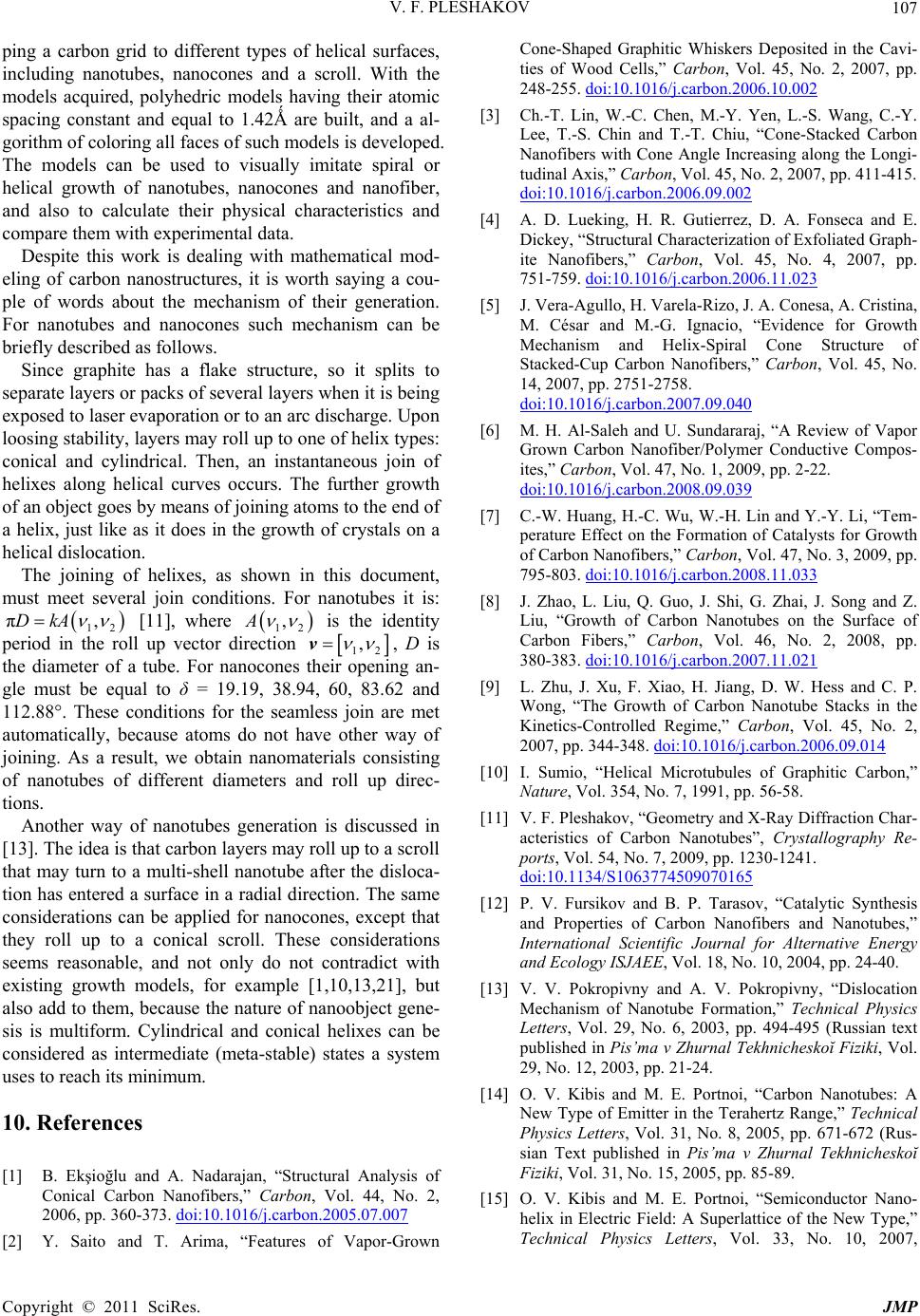 V. F. PLESHAKOV107 ping a carbon grid to different types of helical surfaces, including nanotubes, nanocones and a scroll. With the models acquired, polyhedric models having their atomic spacing constant and equal to 1.42Ǻ are built, and a al- gorithm of coloring all faces of such models is developed. The models can be used to visually imitate spiral or helical growth of nanotubes, nanocones and nanofiber, and also to calculate their physical characteristics and compare them with experimental data. Despite this work is dealing with mathematical mod- eling of carbon nanostructures, it is worth saying a cou- ple of words about the mechanism of their generation. For nanotubes and nanocones such mechanism can be briefly described as follows. Since graphite has a flake structure, so it splits to separate layers or packs of several layers when it is being exposed to laser evaporation or to an arc discharge. Upon loosing stability, layers may roll up to one of helix types: conical and cylindrical. Then, an instantaneous join of helixes along helical curves occurs. The further growth of an object goes by means of joining atoms to the end of a helix, just like as it does in the growth of crystals on a helical dislocation. The joining of helixes, as shown in this document, must meet several join conditions. For nanotubes it is: 12 π,DkA [11], where 12 ,A is the identity period in the roll up vector direction 12 , v, D is the diameter of a tube. For nanocones their opening an- gle must be equal to δ = 19.19, 38.94, 60, 83.62 and 112.88°. These conditions for the seamless join are met automatically, because atoms do not have other way of joining. As a result, we obtain nanomaterials consisting of nanotubes of different diameters and roll up direc- tions. Another way of nanotubes generation is discussed in [13]. The idea is that carbon layers may roll up to a scroll that may turn to a multi-shell nanotube after the disloca- tion has entered a surface in a radial direction. The same considerations can be applied for nanocones, except that they roll up to a conical scroll. These considerations seems reasonable, and not only do not contradict with existing growth models, for example [1,10,13,21], but also add to them, because the nature of nanoobject gene- sis is multiform. Cylindrical and conical helixes can be considered as intermediate (meta-stable) states a system uses to reach its minimum. 10. References [1] B. Ekşioğlu and A. Nadarajan, “Structural Analysis of Conical Carbon Nanofibers,” Carbon, Vol. 44, No. 2, 2006, pp. 360-373. doi:10.1016/j.carbon.2005.07.007 [2] Y. Saito and T. Arima, “Features of Vapor-Grown Cone-Shaped Graphitic Whiskers Deposited in the Cavi- ties of Wood Cells,” Carbon, Vol. 45, No. 2, 2007, pp. 248-255. doi:10.1016/j.carbon.2006.10.002 [3] Ch.-T. Lin, W.-C. Chen, M.-Y. Yen, L.-S. Wang, C.-Y. Lee, T.-S. Chin and T.-T. Chiu, “Cone-Stacked Carbon Nanofibers with Cone Angle Increasing along the Longi- tudinal Axis,” Carbon, Vol. 45, No. 2, 2007, pp. 411-415. doi:10.1016/j.carbon.2006.09.002 [4] A. D. Lueking, H. R. Gutierrez, D. A. Fonseca and E. Dickey, “Structural Characterization of Exfoliated Graph- ite Nanofibers,” Carbon, Vol. 45, No. 4, 2007, pp. 751-759. doi:10.1016/j.carbon.2006.11.023 [5] J. Vera-Agullo, H. Varela-Rizo, J. A. Conesa, A. Cristina, M. César and M.-G. Ignacio, “Evidence for Growth Mechanism and Helix-Spiral Cone Structure of Stacked-Cup Carbon Nanofibers,” Carbon, Vol. 45, No. 14, 2007, pp. 2751-2758. doi:10.1016/j.carbon.2007.09.040 [6] M. H. Al-Saleh and U. Sundararaj, “A Review of Vapor Grown Carbon Nanofiber/Polymer Conductive Compos- ites,” Carbon, Vol. 47, No. 1, 2009, pp. 2-22. doi:10.1016/j.carbon.2008.09.039 [7] C.-W. Huang, H.-C. Wu, W.-H. Lin and Y.-Y. Li, “Tem- perature Effect on the Formation of Catalysts for Growth of Carbon Nanofibers,” Carbon, Vol. 47, No. 3, 2009, pp. 795-803. doi:10.1016/j.carbon.2008.11.033 [8] J. Zhao, L. Liu, Q. Guo, J. Shi, G. Zhai, J. Song and Z. Liu, “Growth of Carbon Nanotubes on the Surface of Carbon Fibers,” Carbon, Vol. 46, No. 2, 2008, pp. 380-383. doi:10.1016/j.carbon.2007.11.021 [9] L. Zhu, J. Xu, F. Xiao, H. Jiang, D. W. Hess and C. P. Wong, “The Growth of Carbon Nanotube Stacks in the Kinetics-Controlled Regime,” Carbon, Vol. 45, No. 2, 2007, pp. 344-348. doi:10.1016/j.carbon.2006.09.014 [10] I. Sumio, “Helical Microtubules of Graphitic Carbon,” Nature, Vol. 354, No. 7, 1991, pp. 56-58. [11] V. F. Pleshakov, “Geometry and X-Ray Diffraction Char- acteristics of Carbon Nanotubes”, Crystallography Re- ports, Vol. 54, No. 7, 2009, pp. 1230-1241. doi:10.1134/S1063774509070165 [12] P. V. Fursikov and B. P. Tarasov, “Catalytic Synthesis and Properties of Carbon Nanofibers and Nanotubes,” International Scientific Journal for Alternative Energy and Ecology ISJAEE, Vol. 18, No. 10, 2004, pp. 24-40. [13] V. V. Pokropivny and A. V. Pokropivny, “Dislocation Mechanism of Nanotube Formation,” Technical Physics Letters, Vol. 29, No. 6, 2003, pp. 494-495 (Russian text published in Pis’ma v Zhurnal Tekhnicheskoĭ Fiziki, Vol. 29, No. 12, 2003, pp. 21-24. [14] O. V. Kibis and M. E. Portnoi, “Carbon Nanotubes: A New Type of Emitter in the Terahertz Range,” Technical Physics Letters, Vol. 31, No. 8, 2005, pp. 671-672 (Rus- sian Text published in Pis’ma v Zhurnal Tekhnicheskoĭ Fiziki, Vol. 31, No. 15, 2005, pp. 85-89. [15] O. V. Kibis and M. E. Portnoi, “Semiconductor Nano- helix in Electric Field: A Superlattice of the New Type,” Technical Physics Letters, Vol. 33, No. 10, 2007, Copyright © 2011 SciRes. JMP  V. F. PLESHAKOV Copyright © 2011 SciRes. JMP 108 878-880 (Russian Text published in Pis’ma v Zhurnal Tekhnicheskoĭ Fiziki, Vol. 33, No. 20, 2007, pp. 57-63. [16] O. V. Kibis, S. V. Malevannyy, L. Hugget, D. G. W. Parfitt and M. E. Portnoi, “Superlattice Properties of Helical Nanostructures in a Transverse Electric Field,” Electromagnetics, Vol. 25, 2005, pp. 425-435. doi:10.1080/02726340590957416 [17] P. L. Chebyshev, “On the Cutting of Our Clothes,” Com- plete works, Moscow, Fizmatgiz, Vol. 5, 1955, pp. 165- 170. [18] E. V. Popov, “Geometrical Modeling of Tent Fabric Structures with the Stretched Grid Method,” Proceedings of the 11 International Conference on Computer Graph- ics&Vision GRAPHICON 2001, UNN, Nizhny Novgorod, Russia, 2001, pp. 138-143. http://www.graphicon.ru/ [19] B. J. Cox and J. M. Hill, “Exact and Approximate Geo- metric Parameters for Carbon Nanotubes Incorporating Curvature,” Carbon, Vol. 45, No. 7, 2007, pp. 1453-1462. doi:10.1016/j.carbon.2007.03.028 [20] B. J. Cox and J. M. Hill, “Geometric Structure of Ul- tra-Small Carbon Nanotubes,” Carbon, Vol. 46, No. 4, 2008, pp. 711-713. doi:10.1016/j.carbon.2007.12.011 [21] Y. E. Lozovik and A. M. Popov, “Formation and Growth of Carbon Nanostructures: Fullerenes, Nanoparticles, Nanotubes and Cones,” Physics-Uspekhi (Advances in Physical Sciences), Vol. 40, 1997, pp. 717-737 (Russian Text published in Uspekhi Fizicheskikh Nauk, Vol. 167, No. 7, 1997, pp. 751-774.
|