Psychology
2011. Vol.2, No.2, 138-142
Copyright © 2011 SciRes. DOI:10.4236/psych.2011.22022
Study on Psychological Crisis Evaluation Combining
Factor Analysis and Neural Networks*
Hui Lin1, Yingbi Zhang1, Hengqing Tong1, Qiaoling Tong2, Dongsheng Liu2
1Department of Mathematics, Wuhan University of Technology, Wuhan, China;
2Department of Electronic Science & Technology, Huazhong University of Science & Technology,
Wuhan, China
Received August 17th, 2010; revised December 16th, 2010; accepted January 15th, 2011.
Effective and rapid psychological crisis evaluation under emergency is the basis to carry out psychological crisis
intervention (PCI). In this paper, based on existing research, an index system to evaluate the state of psycho-
logical crisis is established and the index system is simplified by the model combining factor analysis and neural
networks. Experiments illustrate that the training times, training time and maximum error of the combination
model are 1445, 20.476 (s), 0.0011 respectively while the general neural networks are 5581, 115.610 (s), 0.0090
with 92 samples and the final diagnosis by the combination model are also exact.
Keywords: Psychological Crisis, Evaluation, Inde x S ystem, Factor Analysis, Neural Networks
Introduction
In 1964, American psychologist G. Gaplan originally brought
up psychological crisis (PC). He defined psychological crisis as
the status of psychological unbalance in which individuals
could neither avoid nor cope with sudden or serious life events
(Gaplan, 1964). Once the psychological crisis occurs, the psy-
chological crisis intervention (PCI) is needed immediately to
recalibrate the mental situation to normal level, in case the in-
dividuals fall into a status of suffering, anxiety, coupled with
desperation, autonomic symptoms and behavior disorder.
However, the effective crisis intervention is dependent on ac-
curate evaluation. Through evaluation, the psychologist can
understand the individuals’ crisis situation and their reactions
thus effective crisis intervention can be carried out as soon as
possible.
Myer and Williams (1992) proposed a three-dimensional tri-
age evaluation model which provides a framework for under-
standing individuals’ reactions during a crisis. The model pre-
sumes that reactions to crisis events are seen in three domains:
cognitive, affective and behavioral (Myer, William, Ottens &
Schmidt, 1992). Brende (1998) presented an evaluation model
of phases based on his research on unprecedented and destruc-
tive floods from 1987 to 1998 in USA. In this article he says
that survivors’ predictable emotional and physiological re-
sponses usually process through five phrases over a period of
time toward either resolution or symptom development. To
preclude more severe and chronic symptoms, survivors should
be debriefed by trained professionals within 48 hours (Brende,
1998). Wilson (1999) brought up a person-envi- ronment inter-
actional model to explain the typologies of traumatic events and
stressor dimensions. This model pays attention to comprehen-
sion of stress and its factors as well as the diversity of traumatic
events (Wilson, 1999).
In this article, we propose a novel and effective method to
evaluate PC. Firstly integrating the core idea of Myer and Wil-
liams, we establish an evaluation index system for psychologi-
cal crisis. Further, considering the evaluation should be effec-
tive and valid, we put forward an evaluation model combining
factor analysis and back-propagation neural networks. Through
factor analysis, the intrinsic relationships among indices are
eliminated, and the dimension of these indices is compressed
while enough information is maintained. Moreover, the struc-
ture of the neural networks is simplified. Overall, the accuracy
of networks’ output is improved and the evaluation time is re-
duced.
Establishing Evaluation Index System
Evaluation index system has monitoring function which
adopts one or more rigorous theories to analyze the causal rela-
tionship between individuals and development of crisis accord-
ing to the status of the individuals.
The three-dimensional triage evaluation model proposed by
Myer and Williams is considered to be a simple and rapid
evaluation system. While in a state of emergency, it also re-
quires that the evaluation and the diagnosis should be accurate;
therefore the article starts to establish an evaluation index sys-
tem to evaluate the state of psychological crisis.
When individuals face a crisis, they will conduct a series of
physical and psychological reactions, and the reactions to the
crisis are mainly in physical, emotional, cognitive and behav-
ioral domains. Accordingly, the psychological crisis evaluation
index system can be established from these four domains. The
index system is shown in Table 1.
Using a 90-item self-report symptom inventory (SCL-90) for
reference, we divide each specific index of the evaluation index
system into five levels: not at all, a little bit, moderately, quite a
bit, extremely (Holi, 2003). Each level is assigned a score from
*The project was supported by the National Natural Science Foundation o
f
China (305 70611, 60773210).

H. LIN ET AL. 139
Table 1.
Psychological crisis evalu a tion index system.
reactions indices
gastrointestinal discomfort or diarrhe a, poor appetite
11
C
headache
12
C
Fatigue, insomnia, nightmares, easily s t ar t l ed
13
C
Difficulty in breathi ng or there is a sense of choking or in f arct
14
C
physical
Muscular tension
15
C
scared or suspicious
21
C
Depressed o r sad
22
C
Irritable
23
C
helpless, insensitive
24
C
negative or lonely
25
C
disturbed or nervous
26
C
self-condemned
27
C
Too sensitive or alert , unable to r elax
28
C
emotional
Continuously concerns over the safety of family members, fear of death
29
C
Immersed in the grief of body and mind, leading to changes in memory an d p erception
31
C
Trouble co n centrating and the rel ations expe r ienced between things are ambiguous, leading the ability of making decisions a nd solving
problems affected
32
C
Sometimes be afraid of being mad
33
C
cognitive
Lack of co n fi d ence, easily forgetful, performance degradation, could not turn atten t ion from crisis to other things
34
C
Can not conc entrate on studies or work
41
C
Avoid other people or make oneself feel not lonely in a special way
42
C
Have implemented disruptive behaviors on o n eself or around
43
C
Refused to he l p and it is weak to accept the help
44
C
Behavior is inconsistent with think ing and emotions
45
C
behavioral
Appear typ i cal behaviors which did not occur i n th e past
46
C
one to five respectively. According to the research on reliability
and validity of SCL-90 by Chen Shulin and Li Lingjiang (2003),
the reliability of SCL-90 is good overall, the inter-item consis-
tency reliability of the general scale is 0.97 and those of sub-
scales are over 0.69, the test-retest reliability is over 0.73. The
construct validity of SCL-90 is also good, the correlation coef-
ficients between the general scale and subscales are 0.79-0.92,
and correlation coefficients among subscales are 0.59-0.83
(Chen & Li, 2003).
In SCL-90, the final score is the sum of all scores gained
from each item and the minimum score is 90. Once the final
score is more than 160 points, the examinee requires psycho-
logical counseling or advice. In this evaluation system, we set
the final score to be the average of total scores, lowest score is
1.0, and the highest is 5.0. If the critical average score is more
than 1.77 (160/90), the examinee has a certain mental disorder
and the PCI is required. When the final score is in the interval
of [1.0, 1.77) or [1.77, 2.77) or [2.77, 3.77) or [3.77, 4.77) or
[4.77, 5.0], which indicates the examinees’ five states of psy-
chological crisis.
Factor Analysis
Since the evaluation index system has been established, now
the factor analysis (FA) will be introduced to index compres-
sion.
FA is a widely used method of multivariate statistical analy-
sis. This method is used to describe variability among observed
variables in terms of a potentially lower number of unobserved
variables called factors. If i
Z
is the standardized variable of
i,
Xi
Z
can be expressed a linear combination of factor vari-
ables n
F
and error variable i

, the weight coefficients of
n
F
and i

respectively are and , that is
in
ci d
1
m
iinni
ni
Z
cF d



 (1)
where in is a factor loading expressing the linear correlation
between factor and variable . Estimating factor loadings
are intended to interpret the variation of data as much as possi-
ble. The first main factor has the strongest explanatory power
for variation, while the second main factor is inferior and so on.
cpi
We designed the questionnaires according to the evaluation
index system and sent out 110 questionnaires in the Wenchuan
Earthquake place, we randomly chose the local residents as our
examinees. At last we collected 103 samples, among them only
92 samples are valid, so we use the 92 valid samples to conduct
the data analysis.
Before implementing FA, we firstly adopt Kaiser-Meyer-

H. LIN ET AL. 140
Olkin (KMO) test and Bartlett’s test of sphericity to test the
data whether they are fit for FA. The values of KMO statistic
between 0.7 and 0.8 are good, values between 0.8 and 0.9 are
great and values above 0.9 are superb (Hutcheson & Sofroniou,
1999). For these samples, the value is 0.732, which falls into
the range of being good, so we are confident that the FA is
appropriate for these data.
The Bartlett’s test of sphericity measures the null hypothesis
that the original correlation matrix is an identity matrix. For a
satisfactory FA to proceed, some relationship between variables
are needed, in other words, we want this test to be significant as
a significa nt test tell s us the matrix is not an identity matrix. For
these data, Bartlett’s test is highly significant (p < .001). There-
fore, FA is appropriate (Field, 2005).
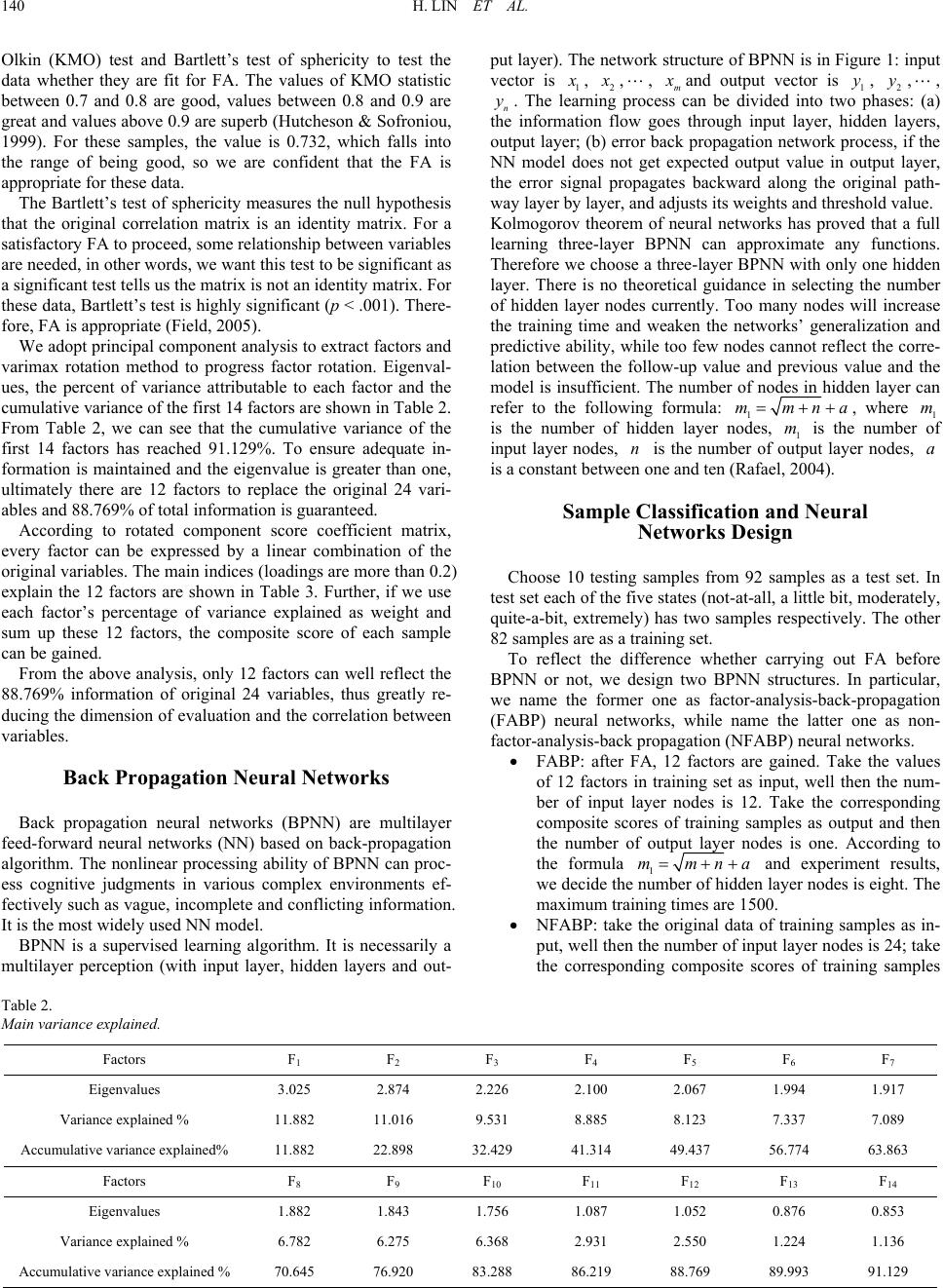
We adopt principal component analysis to extract factors and
varimax rotation method to progress factor rotation. Eigenval-
ues, the percent of variance attributable to each factor and the
cumulative variance of the first 14 factors are shown in Table 2.
From Table 2, we can see that the cumulative variance of the
first 14 factors has reached 91.129%. To ensure adequate in-
formation is maintained and the eigenvalue is greater than one,
ultimately there are 12 factors to replace the original 24 vari-
ables and 88.769% of total information is guaranteed.
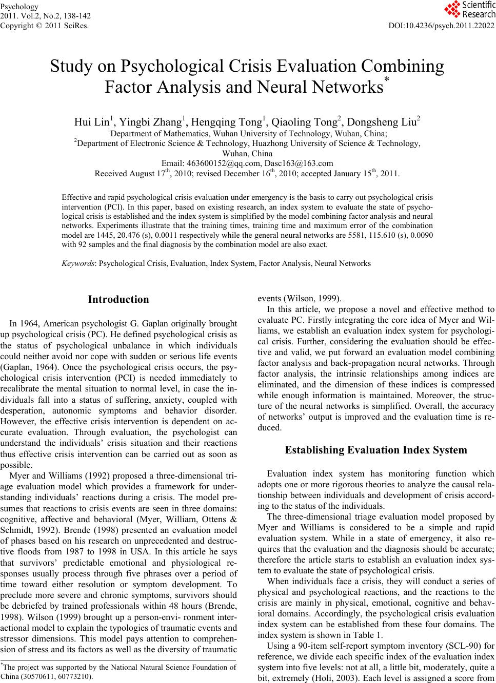
According to rotated component score coefficient matrix,
every factor can be expressed by a linear combination of the
original variables. The main indices (loadings are more than 0.2)
explain the 12 factors are shown in Table 3. Further, if we use
each factor’s percentage of variance explained as weight and
sum up these 12 factors, the composite score of each sample
can be gained.
From the above analysis, only 12 factors can well reflect the
88.769% information of original 24 variables, thus greatly re-
ducing the dimension of evaluation and the correlation between
variables.
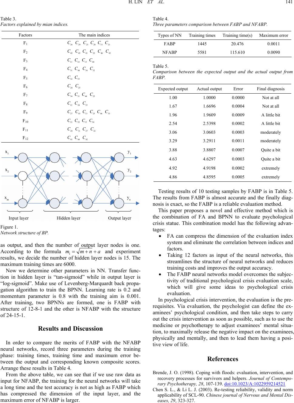
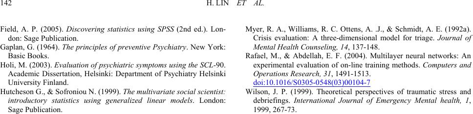
Back Propagation Neural Networks
Back propagation neural networks (BPNN) are multilayer
feed-forward neural networks (NN) based on back-propagation
algorithm. The nonlinear processing ability of BPNN can proc-
ess cognitive judgments in various complex environments ef-
fectively such as vague, incomplete and conflicting information.
It is the most widely used NN model.
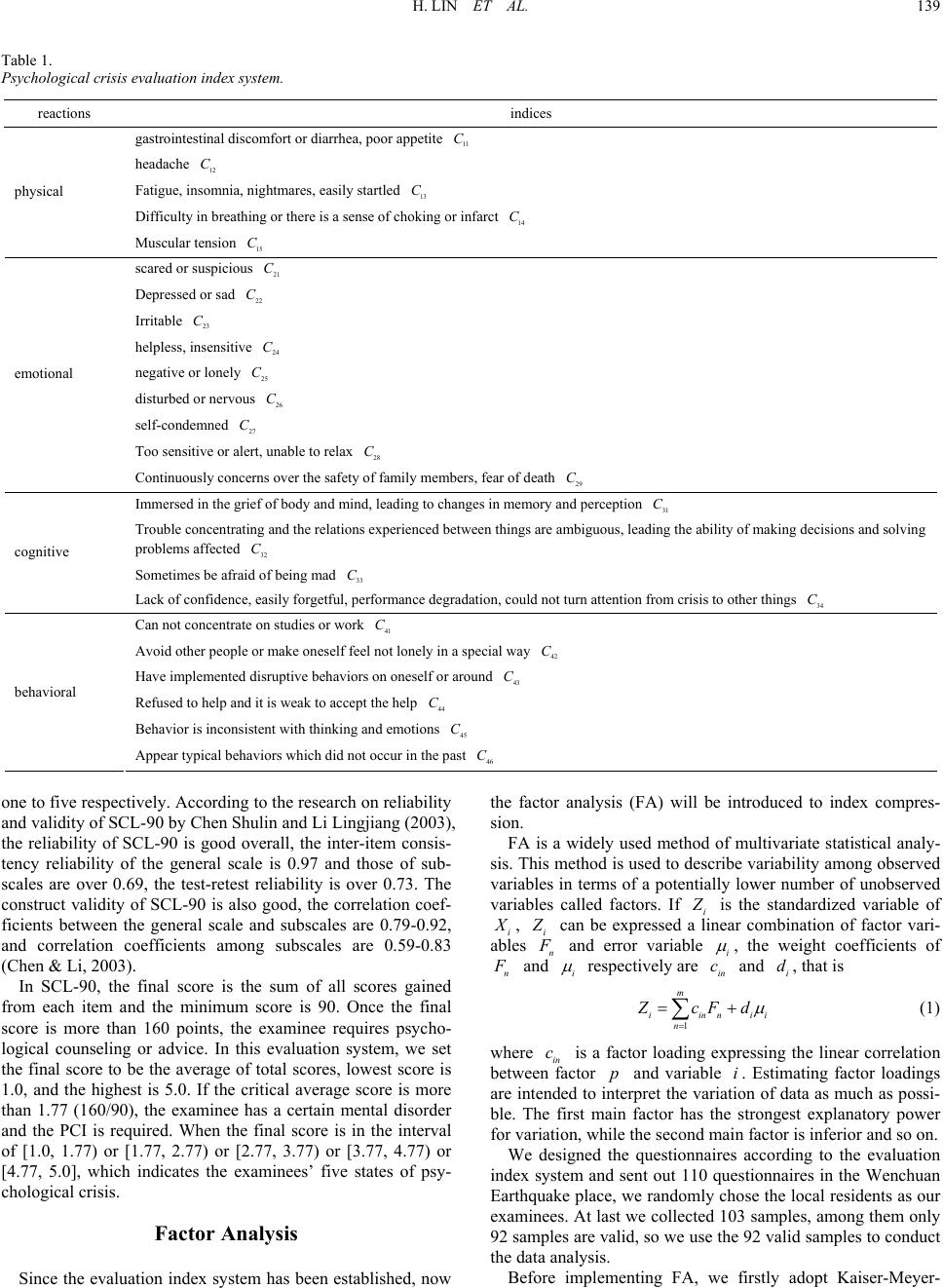
BPNN is a supervised learning algorithm. It is necessarily a
multilayer perception (with input layer, hidden layers and out-
put layer). The network structure of BPNN is in Figure 1: input
vector is 1
x
, 2
x
,, m
x
and output vector is 1, 2,,
n. The learning process can be divided into two phases: (a)
the information flow goes through input layer, hidden layers,
output layer; (b) error back propagation network process, if the
NN model does not get expected output value in output layer,
the error signal propagates backward along the original path-
way layer by layer, and adjusts its weights and threshold value.
y y
y
Kolmogorov theorem of neural networks has proved that a full
learning three-layer BPNN can approximate any functions.
Therefore we choose a three-layer BPNN with only one hidden
layer. There is no theoretical guidance in selecting the number
of hidden layer nodes currently. Too many nodes will increase
the training time and weaken the networks’ generalization and
predictive ability, while too few nodes cannot reflect the corre-
lation between the follow-up value and previous value and the
model is insufficient. The number of nodes in hidden layer can
refer to the following formula: 1
mmna, whe1 m
is the number of hidden layer nodes, 1 m is the number of
input layer nodes, n is the number of output layer nodes, a
is a constant between one and ten (Rafael, 200
 re
4).
Sample Classification and Neural
Networks Design
Choose 10 testing samples from 92 samples as a test set. In
test set each of the five states (not-at-all, a little bit, moderately,
quite-a-bit, extremely) has two samples respectively. The other
82 samples are as a training set.
To reflect the difference whether carrying out FA before
BPNN or not, we design two BPNN structures. In particular,
we name the former one as factor-analysis-back-propagation
(FABP) neural networks, while name the latter one as non-
factor-analysis-back propagation (NFABP) neural networks.
 FABP: after FA, 12 factors are gained. Take the values
of 12 factors in training set as input, well then the num-
ber of input layer nodes is 12. Take the corresponding
composite scores of training samples as output and then
the number of output layer nodes is one. According to
the formula 1
mmna

 and experiment results,
we decide the number of hidden layer nodes is eight. The
maximum training times are 1500.
 NFABP: take the original data of training samples as in-
put, well then the number of input layer nodes is 24; take
the corresponding composite scores of training samples
Table 2.
Main variance explained.
Factors F1 F
2 F 3 F 4 F 5 F 6 F 7
Eigenvalues 3.025 2.874 2.226 2.100 2.067 1.994 1.917
Variance explained % 11.882 11.016 9.531 8.885 8.123 7.337 7.089
Accumulative variance explained% 11.882 22.898 32.429 41.314 49.437 56.774 63.863
Factors F8 F
9 F 10 F 11 F 12 F 13 F 14
Eigenvalues 1.882 1.843 1.756 1.087 1.052 0.876 0.853
Variance explained % 6.782 6.275 6.368 2.931 2.550 1.224 1.136
Accumulative variance explained % 70.645 76.920 83.288 86.219 88.769 89.993 91.129

H. LIN ET AL. 141
Table 3.
Factors explained by mian indices.
Factors The main indices
F1 26
C29 C23 C28 C15 C21 C
F2 42
C45 C41 C22 C46 C43 C
F3 11
C14 C13 C44 C
F4 31
C44 C34 C32 C
F5 32
C33 C
F6 24
C25 C
F7 34
C31 C44 C25 C
F8 12
C24 C33 C
F9 27
C43 C13 C25 C46 C33 C
F10 21
C23 C15 C34 C
F11 24
C31 C27 C22 C
F12 41
C44 C42 C
Figure 1.
Network structure of BP.
as output, and then the number of output layer nodes is one.
According to the formula 1 mmna

 and experiment
results, we decide the number of hidden layer nodes is 15. The
maximum training times are 6000.
Now we determine other parameters in NN. Transfer func-
tion in hidden layer is “tan-sigmoid” while in output layer is
“log-sigmoid”. Make use of Levenberg-Marquardt back propa-
gation algorithm to train the BPNN. Learning rate is 0.2 and
momentum parameter is 0.8 with the training aim is 0.001.
After training, two BPNNs are formed, one is FABP with
structure of 12-8-1 and the other is NFABP with the structure
of 24-15-1.
Results and Discussion
In order to compare the merits of FABP with the NFABP
neural networks, record three parameters during the training
phase: training times, training time and maximum error be-
tween the output and corresponding known composite scores.
Arrange these results in Table 4.
From the above table, we can see that if we use raw data as
input for NFABP, the training for the neural networks will take
a long time and the test accuracy is not as high as FABP which
has compressed the dimension of the input layer, and the
maximum error of NFABP is large r .
Table 4.
Three parameters comparison between FABP and NFABP.
Types of NNTraining timesTraining time(s) Maximum error
FABP 1445 20.476 0.0011
NFABP 5581 115.610 0.0090
Table 5.
Comparison between the expected output and the actual output from
FABP.
Expected o u tputActual output Error Final diagnosis
1.00 1.0000 0.0000 Not at all
1.67 1.6696 0.0004 Not at all
1.96 1.9609 0.0009 A little bit
2.54 2.5398 0.0002 A little bit
3.06 3.0603 0.0003 moderately
3.29 3.2911 0.0011 moderately
3.88 3.8807 0.0007 Quite a bit
4.63 4.6297 0.0003 Quite a bit
4.92 4.9198 0.0002 extremely
4.86 4.8595 0.0005 extremely
Testing results of 10 testing samples by FABP is in Table 5.
The results from FABP is almost accurate and the finally diag-
nosis is exact, so the FABP is a reliable evaluation method.
This paper proposes a novel and effective method which is
the combination of FA and BPNN to evaluate psychological
crisis statue. This combination model has the following advan-
tages:
 FA can compress the dimension of the evaluation index
system and eliminate the correlation between indices and
factors.
 Taking 12 factors as input of the neural networks, this
streamlines the structure of neural networks and reduces
training costs and improves the output accuracy.
 The FABP neural networks model overcomes the subjec-
tivity of traditional psychological crisis evaluation scale,
which will give some ideas to psychological crisis
evaluation.
In psychological crisis intervention, the evaluation is the pre-
requisites. Via evaluation, the psychologist can define the ex-
aminees’ psychological condition, and then take steps to carry
out the crisis intervention as soon as possible, such as to use the
medicine or psychotherapy to adjust examinees’ mental situa-
tion, to maximally release the negative impact on the examinees,
physically and mentally, and then to lead them having a posi-
tive view of life.
References
Brende, J. O. (1998). Coping with floods: evaluation, intervention, and
recovery processes for survivors and helpers. Journal of Contempo-
rary Psychotherapy, 28, 107-139. doi:10.1023/A:1022959214521
Chen S. L., & Li L. J. (2003). Re-testing reliability, validity and norm
applicability of SCL-90. Chinese journal of Nervous and Mental Dis-
eases, 29, 323-327.

H. LIN ET AL. 142
Field, A. P. (2005). Discovering statistics using SPSS (2nd ed.). Lon-
don: Sage Publication.
Gaplan, G. (1964). The principles of preventive Psychiatry. New York:
Basic Books.
Holi, M. (2003). Evaluation of psychiatric symptoms using the SCL-90.
Academic Dissertation, Helsinki: Department of Psychiatry Helsinki
University Finland.
Hutcheson G., & Sofroniou N. (1999). The multivariate social scientist:
introductory statistics using generalized linear models. London:
Sage Publication.
Myer, R. A., Williams, R. C. Ottens, A. .J., & Schmidt, A. E. (1992a).
Crisis evaluation: A three-dimensional model for triage. Journal of
Mental Health Counseling, 14, 137-148.
Rafael, M., & Abdellah, E. F. (2004). Multilayer neural networks: An
experimental evaluation of on-line training methods. Computers and
Operations Research, 31, 1491-1513.
doi:10.1016/S0305-0548(03)00104-7
Wilson, J. P. (1999). Theoretical perspectives of traumatic stress and
debriefings. International Journal of Emergency Mental health, 1,
1999, 267-73.