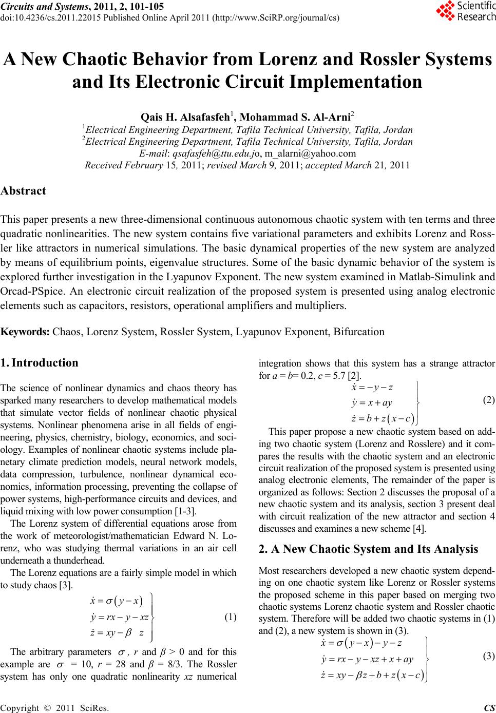Circuits and Systems, 2011, 2, 101-105
doi:10.4236/cs.2011.22015 Published Online April 2011 (http://www.SciRP.org/journal/cs)
A New Chaotic Behavior from Lorenz and Rossler Systems
and Its Electronic Circ uit Implementation
Qais H. Alsafasfeh1, Mohammad S. Al-Arni2
1Electrical Engineering Department, Tafila Technical University, Tafila, Jordan
2Electrical Engineering Department, Tafila Technical University, Tafila, Jordan
Received February 15, 2011; revised March 9, 2011; accepted March 21, 2011
Abstract
This paper presents a new three-dimensional continuous autonomous chaotic system with ten terms and three
quadratic nonlinearities. The new system contains five variational parameters and exhibits Lorenz and Ross-
ler like attractors in numerical simulations. The basic dynamical properties of the new system are analyzed
by means of equilibrium points, eigenvalue structures. Some of the basic dynamic behavior of the system is
explored further investigation in the Lyapunov Exponent. The new system examined in Matlab-Simulink and
Orcad-PSpice. An electronic circuit realization of the proposed system is presented using analog electronic
elements such as capacitors, resistors, operational amplifiers and multipliers.
Keywords: Chaos, Lorenz System, Rossler System, Lyapunov Exponent, Bifurcation
1. Introduction
The science of nonlinear dynamics and chaos theory has
sparked many researchers to develop mathematical models
that simulate vector fields of nonlinear chaotic physical
systems. Nonlinear phenomena arise in all fields of engi-
neering, physics, chemistry, biology, economics, and soci-
ology. Examples of nonlinear chaotic systems include pla-
netary climate prediction models, neural network models,
data compression, turbulence, nonlinear dynamical eco-
nomics, information processing, preventing the collapse of
power systems, high-performance circuits and devices, and
liquid mixing with low power consumption [1-3].
The Lorenz system of differential equations arose from
the work of meteorologist/mathematician Edward N. Lo-
renz, who was studying thermal variations in an air cell
underneath a thunderhead.
The Lorenz equations are a fairly simple model in which
to study chaos [3].

xyx
yrxyxz
zxy z








 




(1)
The arbitrary parameters

, r and β > 0 and for this
example are

= 10, r = 28 and β = 8/3. The Rossler
system has only one quadratic nonlinearity xz numerical
integration shows that this system has a strange attractor
for a = b= 0.2, c = 5.7 [2].

x
yz
yxay
zbzxc


 
 

 




(2)
This paper propose a new chaotic system based on add-
ing two chaotic system (Lorenz and Rosslere) and it com-
pares the results with the chaotic system and an electronic
circuit realization of the proposed system is presented using
analog electronic elements, The remainder of the paper is
organized as follows: Section 2 discusses the proposal of a
new chaotic system and its analysis, section 3 present deal
with circuit realization of the new attractor and section 4
discusses and examines a new scheme [4].
2. A New Chaotic System and Its Analysis
Most researchers developed a new chaotic system depend-
ing on one chaotic system like Lorenz or Rossler systems
the proposed scheme in this paper based on merging two
chaotic systems Lorenz chaotic system and Rossler chaotic
system. Therefore will be added two chaotic systems in (1)
and (2), a new system is shown in (3).



xyxyz
yrxyxzxay
zxy zbzxc






 






(3)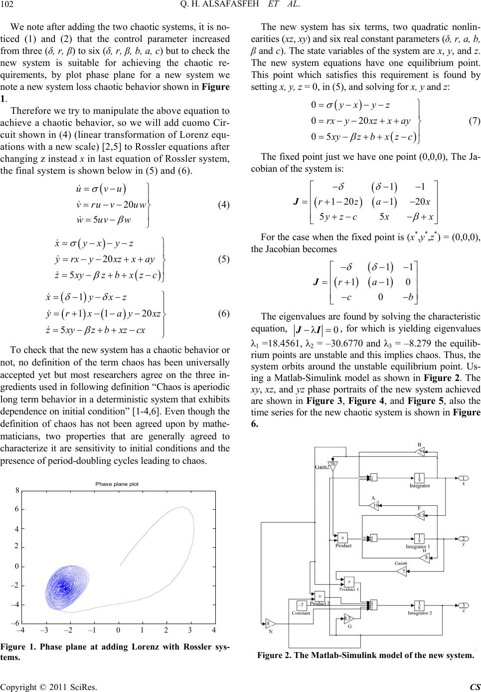

Q. H. ALSAFASFEH ET AL. 102
We note after adding the two chaotic systems, it is no-
ticed (1) and (2) that the control parameter increased
from three (δ, r, β) to six (δ, r, β, b, a, c) but to check the
new system is suitable for achieving the chaotic re-
quirements, by plot phase plane for a new system we
note a new system loss chaotic behavior shown in Figure
1.
Therefore we try to manipulate the above equation to
achieve a chaotic behavior, so we will add cuomo Cir-
cuit shown in (4) (linear transformation of Lorenz equ-
ations with a new scale) [2,5] to Rossler equations after
changing z instead x in last equation of Rossler system,
the final system is shown below in (5) and (6).

20
5
uvu
vruv uw
wuvw


 

 

 



(4)


20
5
xyxyz
yrxy xzxay
zxy zbxzc


 

 






(5)


1
11 20
5
xyxz
yr xayxz
zxyzbxzcx


 

 





(6)
To check that the new system has a chaotic behavior or
not, no definition of the term chaos has been universally
accepted yet but most researchers agree on the three in-
gredients used in following definition “Chaos is aperiodic
long term behavior in a deterministic system that exhibits
dependence on initial condition” [1-4,6]. Even though the
definition of chaos has not been agreed upon by mathe-
maticians, two properties that are generally agreed to
characterize it are sensitivity to initial conditions and the
presence of period-doubling cycles leading to chaos.
-4-3 -2 -10 1 2 34
-6
-4
-2
0
2
4
6
8Phase plane plot
Figure 1. Phase plane at adding Lorenz with Rossler sys-
tems.
The new system has six terms, two quadratic nonlin-
earities (xz, xy) and six real constant parameters (δ, r, a, b,
β and c). The state variables of the system are x, y, and z.
The new system equations have one equilibrium point.
This point which satisfies this requirement is found by
setting x, y, z = 0, in (5), and solving for x, y and z:



0
020
05
yx yz
rxyxzx ay
x
yzbxzc


 

 



(7)
The fixed point just we have one point (0,0,0), The Ja-
cobian of the system is:


11
1201 20
55
rza x
yzcxx







 








J
For the case when the fixed point is (x*,y*,z*) = (0,0,0),
the Jacobian becomes


11
110
0
ra
cb







 








J
The eigenvalues are found by solving the characteristic
equation, 0

JI , for which is yielding eigenvalues
λ1 =18.4561, λ2 = –30.6770 and λ3 = –8.279 the equilib-
rium points are unstable and this implies chaos. Thus, the
system orbits around the unstable equilibrium point. Us-
ing a Matlab-Simulink model as shown in Figure 2. The
xy, xz, and yz phase portraits of the new system achieved
are shown in Figure 3, Figure 4, and Figure 5, also the
time series for the new chaotic system is shown in Figure
6.
Figure 2. The Matlab-Simulink model of the new system.
–
4 –3 –2 –1 0 1 2 3 4
–
6
–
4
–
2
0
2
4
6
8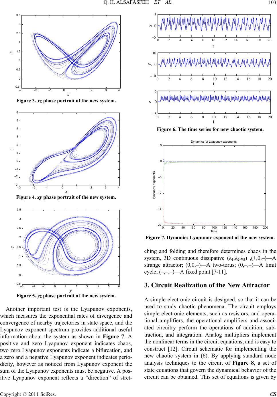

Q. H. ALSAFASFEH ET AL. 103
-3 -2 -1 0 1 2 3 4
-0.5
0
0.5
1
1.5
2
2.5
3
3.5
x
z
Figure 3. xz phase portrait of the new system.
-3 -2 -101234
-3
-2
-1
0
1
2
3
4
5
6
x
y
Figure 4. xy phase portrait of the new system.
-3 -2 -1 0 12 3 4 56
-0. 5
0
0.5
1
1.5
2
2.5
3
3.5
y
z
Figure 5. yz phase portrait of the new system.
Another important test is the Lyapunov exponents,
which measures the exponential rates of divergence and
convergence of nearby trajectories in state space, and the
Lyapunov exponent spectrum provides additional useful
information about the system as shown in Figure 7. A
positive and zero Lyapunov exponent indicates chaos,
two zero Lyapunov exponents indicate a bifurcation, and
a zero and a negative Lyapunov exponent indicates perio-
dicity, however as noticed from Lyapunov exponent the
sum of the Lyapunov exponents must be negative. A pos-
itive Lyapunov exponent reflects a “direction” of stret-
Figure 6. The time series for new chaotic system.
020 4060 80 100 120 140 160 180200
-20
-15
-10
-5
0
5Dynami cs of Ly apunov expo nent s
Time
Ly ap unov e xp onents
Figure 7. Dynamics Lyapunov exponent of the new syste m .
ching and folding and therefore determines chaos in the
system, 3D continuous dissipative (λ1,λ2,λ3) ,(+,0,–)—A
strange attractor; (0,0,–)—A two-torus; (0,–,–)—A limit
cycle; (–,–,–)—A fixed point [7-11].
3. Circuit Realization of the New Attractor
A simple electronic circuit is designed, so that it can be
used to study chaotic phenomena. The circuit employs
simple electronic elements, such as resistors, and opera-
tional amplifiers, the operational amplifiers and associ-
ated circuitry perform the operations of addition, sub-
traction, and integration. Analog multipliers implement
the nonlinear terms in the circuit equations, and is easy to
construct [12]. Circuit schematic for implementing the
new chaotic system in (6). By applying standard node
analysis techniques to the circuit of Figure 8, a set of
state equations that govern the dynamical behavior of the
circuit can be obtained. This set of equations is given by
–3 –2 –1 0 1 2 3 4
–0.5
–1
–2
–3
–3 –2 –1 0 1 2 3 4
–3 –2 –1 0 1 2 3 4 5 6
–0.5
–5
–10
–15
–20
x
x
y
z y z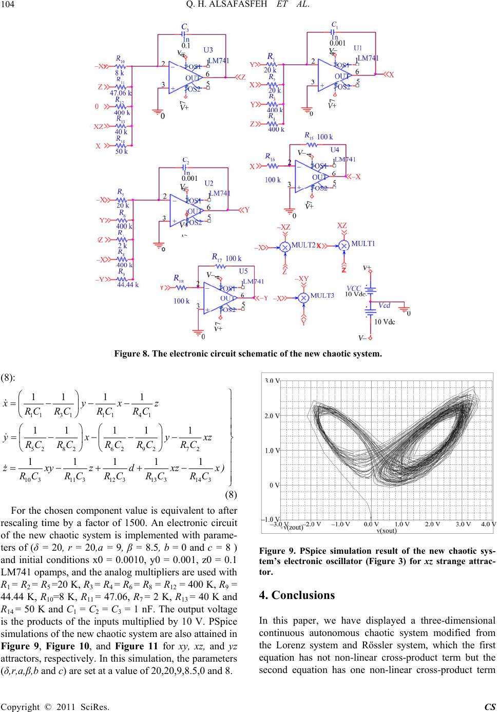

Q. H. ALSAFASFEH ET AL. 104
Figure 8. The electronic circuit schematic of the new chaotic system.
(8):
11 311141
52 8262 9272
10 311312 313 314 3
1111
1111 1
11111
xyxz
RCRCRCRC
yxyxz
RC RCRC RCRC
zxyzdxzx)
RCRCRCRCRC


 







 











(8)
For the chosen component value is equivalent to after
rescaling time by a factor of 1500. An electronic circuit
of the new chaotic system is implemented with parame-
ters of (δ = 20, r = 20,a = 9, β = 8.5, b = 0 and c = 8 )
and initial conditions x0 = 0.0010, y0 = 0.001, z0 = 0.1
LM741 opamps, and the analog multipliers are used with
R1 = R2 = R5 =20 K, R3 = R4 = R6 = R8 = R12 = 400 K, R9 =
44.44 K, R10=8 K, R11 = 47.06, R7 = 2 K, R13 = 40 K and
R14 = 50 K and C1 = C2 = C3 = 1 nF. The output voltage
is the products of the inputs multiplied by 10 V. PSpice
simulations of the new chaotic system are also attained in
Figure 9, Figure 10, and Figure 11 for xy, xz, and yz
attractors, respectively. In this simulation, the parameters
(δ,r,a,β,b and c) are set at a value of 20,20,9,8.5,0 and 8.
Figure 9. PSpice simulation result of the new chaotic sys-
tem’s electronic oscillator (Figure 3) for xz strange attrac-
tor.
4. Conclusions
In this paper, we have displayed a three-dimensional
continuous autonomous chaotic system modified from
the Lorenz system and Rössler system, which the first
equation has not non-linear cross-product term but the
second equation has one non-linear cross-product term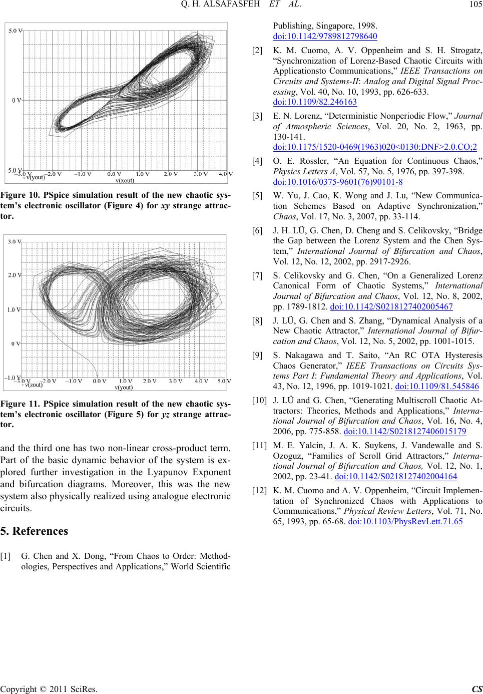

Q. H. ALSAFASFEH ET AL. 105
Figure 10. PSpice simulation result of the new chaotic sys-
tem’s electronic oscillator (Figure 4) for xy strange attrac-
tor.
Figure 11. PSpice simulation result of the new chaotic sys-
tem’s electronic oscillator (Figure 5) for yz strange attrac-
tor.
and the third one has two non-linear cross-product term.
Part of the basic dynamic behavior of the system is ex-
plored further investigation in the Lyapunov Exponent
and bifurcation diagrams. Moreover, this was the new
system also physically realized using analogue electronic
circuits.
5. References
[1] G. Chen and X. Dong, “From Chaos to Order: Method-
ologies, Perspectives and Applications,” World Scientific
Publishing, Singapore, 1998.
doi:10.1142/9789812798640
[2] K. M. Cuomo, A. V. Oppenheim and S. H. Strogatz,
“Synchronization of Lorenz-Based Chaotic Circuits with
Applicationsto Communications,” IEEE Transactions on
Circuits and Systems-II: Analog and Digital Signal Proc-
essing, Vol. 40, No. 10, 1993, pp. 626-633.
doi:10.1109/82.246163
[3] E. N. Lorenz, “Deterministic Nonperiodic Flow,” Journal
of Atmospheric Sciences, Vol. 20, No. 2, 1963, pp.
130-141.
doi:10.1175/1520-0469(1963)020<0130:DNF>2.0.CO;2
[4] O. E. Rossler, “An Equation for Continuous Chaos,”
Physics Letters A, Vol. 57, No. 5, 1976, pp. 397-398.
doi:10.1016/0375-9601(76)90101-8
[5] W. Yu, J. Cao, K. Wong and J. Lu, “New Communica-
tion Schemes Based on Adaptive Synchronization,”
Chaos, Vol. 17, No. 3, 2007, pp. 33-114.
[6] J. H. LÜ, G. Chen, D. Cheng and S. Celikovsky, “Bridge
the Gap between the Lorenz System and the Chen Sys-
tem,” International Journal of Bifurcation and Chaos,
Vol. 12, No. 12, 2002, pp. 2917-2926.
[7] S. Celikovsky and G. Chen, “On a Generalized Lorenz
Canonical Form of Chaotic Systems,” International
Journal of Bifurcation and Chaos, Vol. 12, No. 8, 2002,
pp. 1789-1812. doi:10.1142/S0218127402005467
[8] J. LÜ, G. Chen and S. Zhang, “Dynamical Analysis of a
New Chaotic Attractor,” International Journal of Bifur-
cation and Chaos, Vol. 12, No. 5, 2002, pp. 1001-1015.
[9] S. Nakagawa and T. Saito, “An RC OTA Hysteresis
Chaos Generator,” IEEE Transactions on Circuits Sys-
tems Part I: Fundamental Theory and Applications, Vol.
43, No. 12, 1996, pp. 1019-1021. doi:10.1109/81.545846
[10] J. LÜ and G. Chen, “Generating Multiscroll Chaotic At-
tractors: Theories, Methods and Applications,” Interna-
tional Journal of Bifurcation and Chaos, Vol. 16, No. 4,
2006, pp. 775-858. doi:10.1142/S0218127406015179
[11] M. E. Yalcin, J. A. K. Suykens, J. Vandewalle and S.
Ozoguz, “Families of Scroll Grid Attractors,” Interna-
tional Journal of Bifurcation and Chaos, Vol. 12, No. 1,
2002, pp. 23-41. doi:10.1142/S0218127402004164
[12] K. M. Cuomo and A. V. Oppenheim, “Circuit Implemen-
tation of Synchronized Chaos with Applications to
Communications,” Physical Review Letters, Vol. 71, No.
65, 1993, pp. 65-68. doi:10.1103/PhysRevLett.71.65