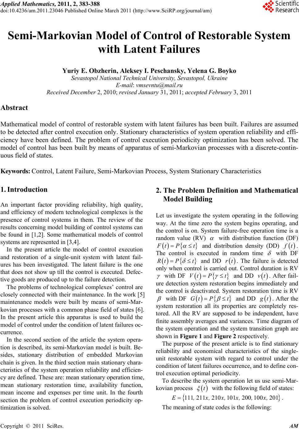Applied Mathematics, 2011, 2, 383-388
doi:10.4236/am.2011.23046 Published Online March 2011 (http://www.SciRP.org/journal/am)
Semi-Markovian Model of Control of Restorable System
with Latent Failures
Yuriy E. Obzherin, Aleksey I. Peschansky, Yelena G. Boyko
Sevastopol National Technical University, Sevastopol, Ukraine
Received December 2, 2010; revised January 31, 2011; accepted February 3, 2011
Abstract
Mathematical model of control of restorable system with latent failures has been built. Failures are assumed
to be detected after control execution only. Stationary characteristics of system operation reliability and effi-
ciency have been defined. The problem of control execution periodicity optimization has been solved. The
model of control has been built by means of apparatus of semi-Markovian processes with a discrete-contin-
uous field of states.
Keywords: Control, Latent Failure, Semi-Markovian Process, System Stationary Characteristics
1. Introduction
An important factor providing reliability, high quality,
and efficiency of modern technological complexes is the
presence of control systems in them. The review of the
results concerning model building of control systems can
be found in [1,2]. Some mathematical models of control
systems are represented in [3,4].
In the present article the model of control execution
and restoration of a single-unit system with latent fail-
ures has been investigated. The latent failure is the one
that does not show up till th e control is executed. Defec-
tive goods are produced up to the failure detection.
The problems of technological complexes’ control are
closely connected with their maintenance. In the work [5]
maintenance models were built by means of semi-Mar-
kovian processes with a common phase field of states [6].
In the present article this apparatus is used to build the
model of control under the cond ition of latent failures oc-
currence.
In the second section of the article the system opera-
tion is described, its semi-Markovian model is built. Be-
sides, stationary distribution of embedded Markovian
chain is given. In the third sectio n main stationary chara-
cteristics of the system operation reliability and efficien-
cy are defined. These are: mean stationary operation time,
mean stationary restoration time, availability function,
mean income and expenses per time unit. In the fourth
section the problem of control execution periodicity op-
timization is solved.
2. The Problem Definition and Mathematical
Model Building
Let us investigate the system operating in the following
way. At the time zero the system begins operating, and
the control is on. System failure-free operation time is a
random value (RV)

with distribution function (DF)




F
tP t 

 and distribution density (DD)


f
t.
The control is executed in random time

with DF




Rt Pt 

 and DD


rt. The failure is detected
only when control is carried out. Control duration is RV

with DF




Vt Pt 

 and DD


vt. After fail-
ure detection system restoration begins immediately and
the control is deactivated. System restoration time is RV

with DF




Gt Pt 

 and DD

g
t. After the
system restoration all its properties are completely res-
tored. All the RV are supposed to be independent, have
finite assembly averages and variances. Time diagram of
the system operation and the system transition graph are
shown in Figure 1 and Figure 2 respectively.
The purpose of the present article is to find stationary
reliability and economical characteristics of the single-
unit restorable system with regard to control under the
condition of latent failures occurren ce, and to define con-
trol execution optimal periodicity.
To describe the system operation let us use semi-Mar-
kovian process


t

with the following field of states:


111211210101200 100201E,x,x, x,,x,.
The meaning of state codes is the following: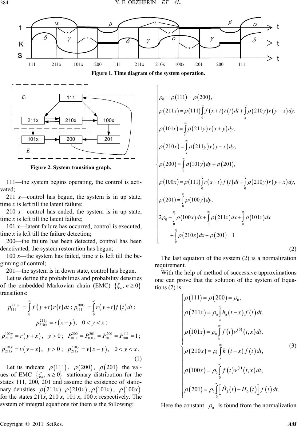

Y. E. OBZHERIN ET AL. 384
211x 110










110
222
110 211x
101x
210x 100x201 222
t
t
t
1
K
x
x
x
x
x

S
111 211x 101x 200 111 211x 210x 100x 201 200 111
Figure 1. Time diagram of the system operation.
111
211x
101x
210x
200
100x
201
Е
+

E
Figure 2. System transition graph.
111—the system begins operating, the control is acti-
vated;
211 х—control has begun, the system is in up state,
time х is left till the latent failure;
210 х—control has ended, the system is in up state,
time х is left till the latent failure;
101 х—latent failure has occurred, control is executed,
time х is left till the failure detection;
200—the failure has been detected, control has been
deactivated, the system restoration has begun;
100 х—the system has failed, time х is left till the be-
ginning of control;
201—the system is in down state, control has begun.
Let us define the probabilities and probability densities
of the embedded Markovian chain (EMC)

0
n,n
 
transitions:

211
111 0
y
pfytrtdt


;

100
111 0
y
prytftdt


;

211
210 ,
y
x
prxy 0
y
x;

100
210y x
pryx, 0y; 200201200 111
101100201200 1
xx
PPPP;

101
211y x
pvyx, 0y;

210
211 ,
y
x
pvxy 0
y
x

.
(1)
Let us indicate

111  ,


200  ,

201  the val-
ues of EMC

,0
nn
  stationary distribution for the
states 111, 200, 201 and assume the existence of statio-
nary densities

211
х
 ,

210
х
 ,

101
х
 ,


100
х

for the states 211x, 210 x, 101 x, 100 x respectively. The
system of integral equations for th em is the following:
 

  
 
 
 

  
0
0
0
0
00
0
0000
111200 ,
211 111210,
101 211,
210 211,
200101201 ,
100 111210,
201100 ,
2 100211101
x
x
x
f xtrtdtyryxdy
xyvxydy
xyvyxdy
ydy
x
rxt ftdtyryxdy
ydy
xdxxdx xdx
 
 


 
 

 








 



 









 
0
210201 1xdx 



































(2)
The last equation of the system (2) is a normalization
requirement.
With the help of method of successive approximations
one can prove that the solution of the system of Equa-
tions (2) is:




 
 


 
 


 
0
00
0
00
01
1
00
01 0
0
111200 ,
211 ,
101, ,
210 ,
100,,
ˆ
201 .
x
x
хht xftdt
xfttxdt
хht xftdt
xfttxdt
H
tHtftdt
 










 

























(3)
Here the con sta n t 0

is found from the normalization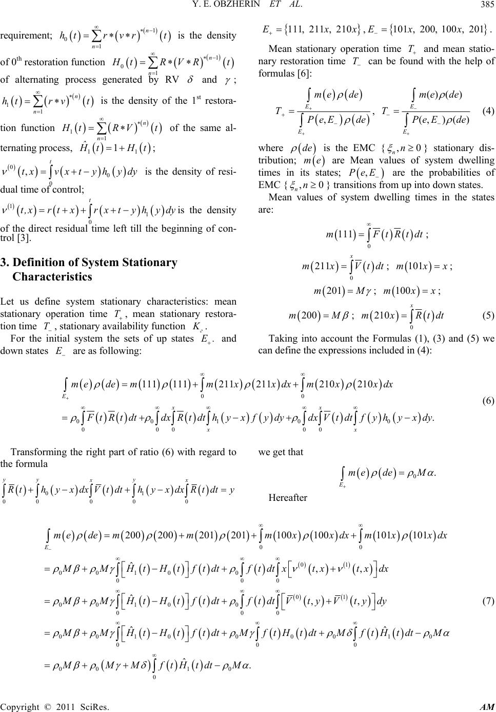

Y. E. OBZHERIN ET AL. 385
requirement;
 


1
01
n
n
htr vrt



 is the density
of 0th restoration function
 


1
01
n
n
H
tRVRt




of alternating process generated by RV

and

;
 


11
n
n
htrv t



 is the density of the 1st restora-
tion function
 


11
n
n
H
tRVt



 of the same al-
ternating process,
 
11
1
ˆ
H
tHt ;

 
00
0
,t txvx tyhydy  
 is the density of resi-
dual time of control;

 
11
0
t
t,xr txrxty hy dy   
is the density
of the direct residual time left till the beginning of con-
trol [3].
3. Definition of System Stationary
Characteristics
Let us define system stationary characteristics: mean
stationary operation time T, mean stationary restora-
tion time T, statio nary availability function г
K
.
For the initial system the sets of up states E.

and
down states E are as following:


111, 211, 210Ех
х
,

101, 200, 100, 201Eхх
.
Mean stationary operation time T and mean statio-
nary restoration time T

can be found with the help of
formulas [6]:
 

,
Е
E
me de
Т
PeE de








,
() ()
(,) ()
E
E
me de
TPeE de








 (4)
where


de  is the EMC {,0
nn

} stationary dis-
tribution;


me are Mean values of system dwelling
times in its states;


,PeE
 are the probabilities of
EMC {,0
nn

} transitions from up into down states.
Mean values of system dwelling times in the states
are:
  
0
111mFtRtdt

;
 
0
211 x mxVtdt;

101mxx;


201m
М

;

100mx
х
;


200m
М

;
 
0
210 x mxRtdt (5)
Taking into account the Formulas (1), (3) and (5) we
can define the expressions included in (4):
 
 
00
001 00
000 00
111 111211211210210
.
E
xx
xx
m edemmxx dxmxxdx
F
tRtdtdxRtdthyxf ydydxVtdt f yhyxdy
 
 



 
 

 
(6)
Transforming the right part of ratio (6) with regard to
the formula
  
01
00000
yy y xx
R
thyxdxVt dthyx dxRtdty 

we get that
 
0.
E
me deM





Hereafter
  
 




 




 
00
01
00 100
000
01
00 100
000
00 10
200200201 201100100101101
ˆ,,
ˆ,,
ˆ
E
mede mmmxxdxmxxdx
MMHtHtftdtftdtxtx txdx
MMHtHtftdtft dtVt yVt ydy
MMHtHtf
 

 





 
 
  
 
 
  
 

 




 
 
00010
000
001 0
0
ˆ
ˆ.
tdtMf tHtdtMf tHtdtM
MMMftHtdtM


 



 


(7)

Y. E. OBZHERIN ET AL. 386
The identity



 
01 01
0
ˆ
Vt,yVt,ydyM HtM Htt





has been used while transforming the expression (7).
Then







01
0
ˆ M.
E
me de
MM fzHzdz


 


 



 (8)
Hereafter
 
   
00
0 0
00 0
,111111,211211 ,210210,
211210 .
E
PeEdePExP xEdxxPxEdx
RtftdtVxx dxRxx dx
 



 
 
 
  

 
Thus, mean stationary operation time T and mean
stationary restoration time T are defined with the help
of formulas ,TM



1
0
ˆ
TMMM MftHtdt  

.
Stationary availability function is defined by the ra-
tio г
Т
К
ТТ


. We get

1
0
ˆ
() ()
г
M
К
M
MM ftHtdt





. (9)
It is necessary to note the probability essence of the
functional in the Formula (9):
 
1
0
ˆ
f
tH tdt

 is an
average value of controls executed before the latent fail-
ure detection.
Important characteristics for system operation quality
testing are economical criteria, such as mean income S
per unit of calendar time and mean expenses C per time
unit of system’s up state. To define them let us use the
formulas [7]:






 
s
E
E
mеfеdе
Smеdе



,
 


 
c
E
E
mеfеdе
Cmеdе




. (10)
Here




sc
fе,fe are the functions defining in-
come and expenses in each state respectively.
Let c1 be the income received per time unit of sys-
tem’s up state; c2–expenses per time unit of restoration;
c3–expenses per time unit of control; c4 are wastes
caused by defective goods p er ti me un it of latent failure.
For the given system the functions



sc
fе,f e are
the following:





1
13
2
34
4
,111, 210,
,211,
, 220,
,101, 201,
,100,
s
се x
cce х
fe се
сcеx
cеx
 



 

 









3
2
34
4
0,111, 210,
,211 ,
,220,
,101, 201,
,100.
c
еx
ce х
fe се
сcеx
cеx
 









(11)
Using Formulas (3), (5), (8) and (11) we will define the functionals included into the expressions (10):
    
     
 
 
113 1
00
234344
00
10 20 401
0
30100
00
111 111211211210210
200 200201101100
ˆ
ˆ
s
E
me fedecmccxmxdxcxmxdx
cmcc Mccxxdxcxxdx
cMcMcM MftHtdtM
cMHtHtftdtftdth tx
 

  





 


 










 


 

 
0
0000
0142341
0
,
ˆ
tx
dxVt dtft dt Vtxdx
ccMcMcM cM MftHtdt 






 




(12)

Y. E. OBZHERIN ET AL. 387
  
 
 
 

 
23 3
0
3444
000
401 20
0
0
30 010
00000
200211 211201
101101100 201
ˆ
ˆ
,
c
E
tx
mefedecMcxmx dxcM
cxxdxcxxdxcxxdx cM
cMMftHtdtMcM
cft dthtxdxVtdtft dtVtxdxMHtHtft dt
 

 





 


 



 





  
0
0243441
0
ˆ.cMcMccMcMftHt dt
 


 
 
 








(13)
When transforming the ratios (12), (13), the identity


 
0
0 0
000000
tx
f
t dthtxdxVtdtft dtVt,xdxMftHt dt 

 
 
was taken into account. Consequently, income per calendar time unit can be calculated by means of the formula:
   
 
1423 41
0
1
0
ˆ
ccMcMcM cMMftHtdt
S
ˆ
MMMftHtdt
 








(14)
Expenses per time unit of system’s good state are de-
fined by the formul a:
  
2344 14
0
ˆ.
C
MMM
ccccftHtdtc
MMM





 



(15)
Let us write down the formulas for the definition of sta-
tionary reliability and economical characteristics of the
system investigated under the condition that time periods
between control execution are non-random values 0

.
Taking into account that in this case



1Rtt ,


where const

, the ratio (9) transforms into:
 

10
1
г
n
n
М
К.
M
MFznvdz

 




 



(16)
Under the assumption that the control duration is
non-random as well:




1,Vtt hwhere h const

.
Then Formulas (9), (14) and (15) look like this:
  
0
г
n
М
К
M
hFn h

 



 
, (17)
 



  
1423440
0
n
n
ccM cMcchcFnh
S
MhFnh
 
 






 

 (18)
 

2344 4
0n
C
Mh
ccccFnhc
MMM







 



(19)
One should note that if 0h and 0

 we get
characteristics for the system with continuous control
[6]:
г
М
К
М
М



, 12 ,
cMc M
SMM




 2
M
Cc
M


.
(20)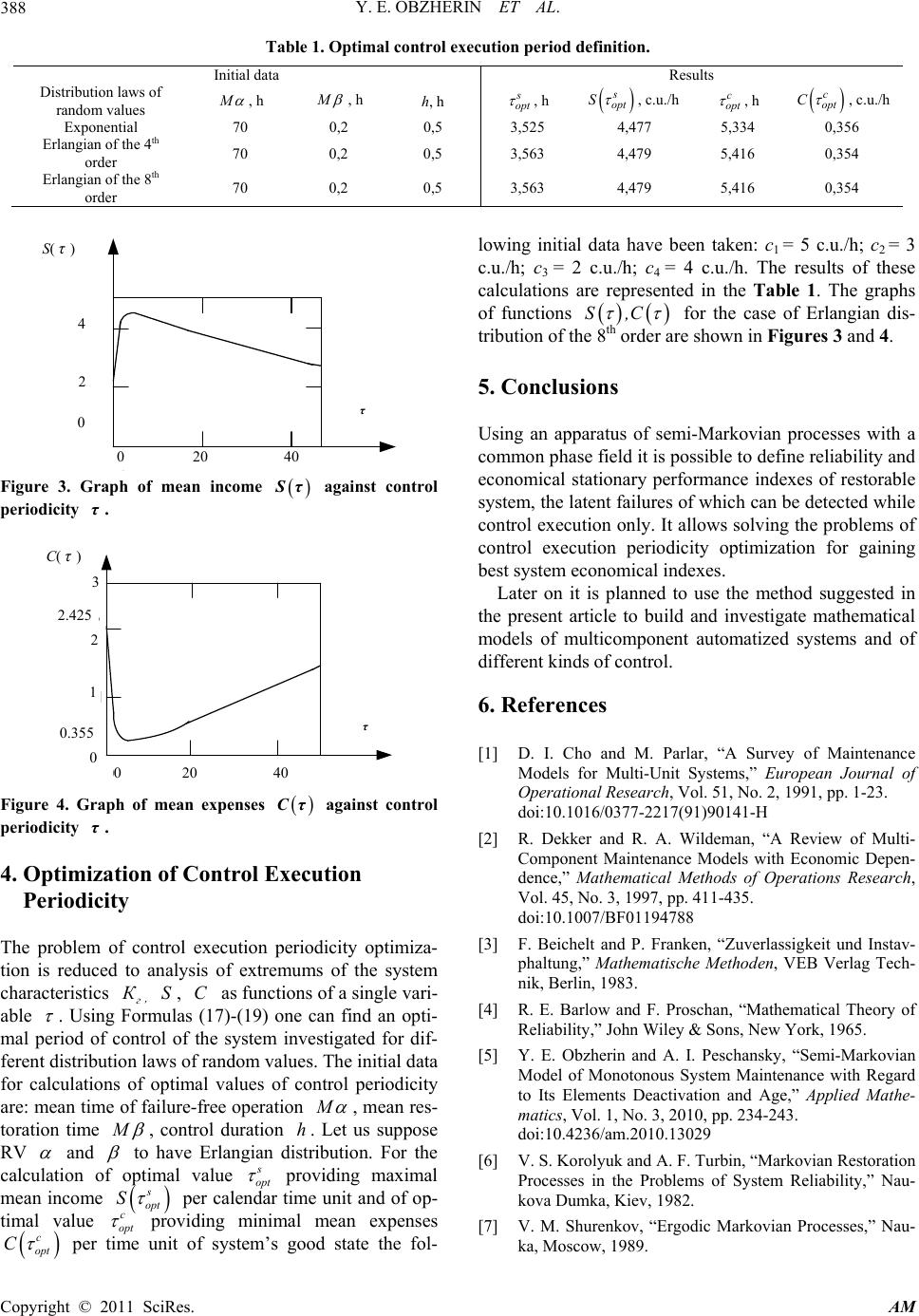

Y. E. OBZHERIN ET AL. 388
Table 1. Optimal control execution period definition.
Initial data Results
Distribution laws of
random values
M

, h M

, h h, h
s
opt

, h


s
opt
S  , c.u./h c
opt

, h


c
opt
C  , c.u./h
Exponential 70 0,2 0,5 3,525 4,477 5,334 0,356
Erlangian of the 4th
order 70 0,2 0,5 3,563 4,479 5,416 0,354
Erlangian of the 8th
order 70 0,2 0,5 3,563 4,479 5,416 0,354
)(  S

4
2
0
020 40
Figure 3. Graph of mean income

Sτ against control
periodicity τ.
3
2
1
0020 40

)(

C
0,355
2,425
Figure 4. Graph of mean expenses

Cτ against control
periodicity τ.
4. Optimization of Control Execution
Periodicity
The problem of control execution periodicity optimiza-
tion is reduced to analysis of extremums of the system
characteristics г
К
, S, C as functions of a single vari-
able

. Using Formulas (17)-(19) one can find an opti-
mal period of control of the system investigated for dif-
ferent distribution laws of random values. The initial data
for calculations of optimal values of control periodicity
are: mean time of failure-free operation
M

, mean res-
toration time
M

, control duration h. Let us suppose
RV

and

to have Erlangian distribution. For the
calculation of optimal value
s
opt

providing maximal
mean income

s
opt
S  per calendar time unit and of op-
timal value c
opt

providing minimal mean expenses

c
opt
C 
per time unit of system’s good state the fol-
lowing initial data have been taken: с1 = 5 c.u./h; с2 = 3
c.u./h; с3 = 2 c.u./h; с4 = 4 c.u./h. The results of these
calculations are represented in the Table 1. The graphs
of functions




S,C

 for the case of Erlangian dis-
tribution of the 8th order are shown in Figures 3 and 4.
5. Conclusions
Using an apparatus of semi-Markovian processes with a
common phase field it is p ossible to define reliability an d
economical stationary performance indexes of restorable
system, the latent failures of which can be detected while
control executio n only. It allows solving the problems of
control execution periodicity optimization for gaining
best system economical indexes.
Later on it is planned to use the method suggested in
the present article to build and investigate mathematical
models of multicomponent automatized systems and of
different kinds of control.
6. References
[1] D. I. Cho and M. Parlar, “A Survey of Maintenance
Models for Multi-Unit Systems,” European Journal of
Operational Research, Vol. 51, No. 2, 1991, pp. 1-23.
doi:10.1016/0377-2217(91)90141-H
[2] R. Dekker and R. A. Wildeman, “A Review of Multi-
Component Maintenance Models with Economic Depen-
dence,” Mathematical Methods of Operations Research,
Vol. 45, No. 3, 1997, pp. 411-435.
doi:10.1007/BF01194788
[3] F. Beichelt and P. Franken, “Zuverlassigkeit und Instav-
phaltung,” Mathematische Methoden, VEB Verlag Tech-
nik, Berlin, 1983.
[4] R. E. Barlow and F. Proschan, “Mathematical Theory of
Reliability,” John Wiley & Sons, New York, 1965.
[5] Y. E. Obzherin and A. I. Peschansky, “Semi-Markovian
Model of Monotonous System Maintenance with Regard
to Its Elements Deactivation and Age,” Applied Mathe-
matics, Vol. 1, No. 3, 2010, pp. 234-243.
doi:10.4236/am.2010.13029
[6] V. S. Korolyuk and A. F. Turbin, “Markovian Restoration
Processes in the Problems of System Reliability,” Nau-
kova Dumka, Kiev, 1982.
[7] V. M. Shurenkov, “Ergodic Markovian Processes,” Nau-
ka, Moscow, 1989.
0 20 40
0
2
4
S(τ)
τ
τ
0 20 40
C(τ)
3
2.425
2
1
0.355
0