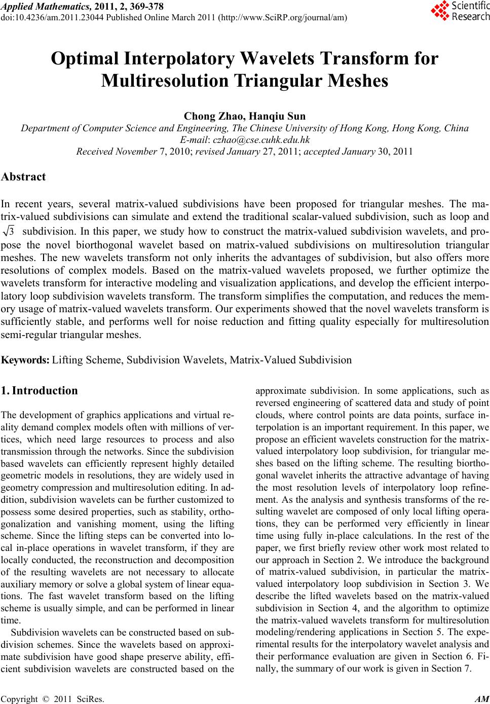Applied Mathematics, 2011, 2, 369-378
doi:10.4236/am.2011.23044 Published Online March 2011 (http://www.SciRP.org/journal/am)
Optimal Interpolatory Wavelets Transform for
Multir esolution Triangular Meshes
Chong Zhao, Hanqiu Sun
Department of Computer Science and Engineering, The Chinese University of Hong Kong, Hong Kong, China
Received November 7, 2010; revised January 27, 2011; accepted January 30, 2011
Abstract
In recent years, several matrix-valued subdivisions have been proposed for triangular meshes. The ma-
trix-valued subdivisions can simulate and extend the traditional scalar-valued subdivision, such as loop and
3 subdivision. In this paper, we study how to construct the matrix-valued subdivision wavelets, and pro-
pose the novel biorthogonal wavelet based on matrix-valued subdivisions on multiresolution triangular
meshes. The new wavelets transform not only inherits the advantages of subdivision, but also offers more
resolutions of complex models. Based on the matrix-valued wavelets proposed, we further optimize the
wavelets transform for interactive modeling and visualization applications, and develop the efficient interpo-
latory loop subdivision wavelets transform. The transform simplifies the computation, and reduces the mem-
ory usage of matrix-valued wavelets transform. Our experiments showed that the novel wavelets transform is
sufficiently stable, and performs well for noise reduction and fitting quality especially for multiresolution
semi-regular triangular meshes.
Keywords: Lifting Scheme, Subdivision Wavelets, Matrix-Valued Subdivision
1. Introduction
The development of graphics applications and virtual re-
ality demand complex models often with millions of ver-
tices, which need large resources to process and also
transmission through the networks. Since the subdivision
based wavelets can efficiently represent highly detailed
geometric models in resolutions, they are widely used in
geometry compression and multiresolution editing. In ad-
dition, subdivision wavelets can be further customized to
possess some desired properties, such as stability, ortho-
gonalization and vanishing moment, using the lifting
scheme. Since the lifting steps can be converted into lo-
cal in-place operations in wavelet transform, if they are
locally conducted, the reconstruction and decomposition
of the resulting wavelets are not necessary to allocate
auxiliary memory or solve a global system of linear equa-
tions. The fast wavelet transform based on the lifting
scheme is usually simple, and can be performed in linear
time.
Subdivision wavelets can be constructed based on sub-
division schemes. Since the wavelets based on approxi-
mate subdivision have good shape preserve ability, effi-
cient subdivision wavelets are constructed based on the
approximate subdivision. In some applications, such as
reversed engineering of scattered data and study of point
clouds, where control points are data points, surface in-
terpolation is an important requirement. In this paper, we
propose an efficient wavelets construction for the matrix-
valued interpolatory loop subdivision, for triangular me-
shes based on the lifting scheme. The resulting biortho-
gonal wavelet inherits the attractive advantage of having
the most resolution levels of interpolatory loop refine-
ment. As the analysis and synthesis transforms of the re-
sulting wavelet are composed of only local lifting opera-
tions, they can be performed very efficiently in linear
time using fully in-place calculations. In the rest of the
paper, we first briefly review other work most related to
our approach in Section 2. We introduce the background
of matrix-valued subdivision, in particular the matrix-
valued interpolatory loop subdivision in Section 3. We
describe the lifted wavelets based on the matrix-valued
subdivision in Section 4, and the algorithm to optimize
the matrix-valued wavelets transform for multiresolution
modeling/rendering applications in Section 5. The expe-
rimental results for the interpolatory wavelet analysis and
their performance evaluation are given in Section 6. Fi-
nally, the summary of our work is given in Section 7.

C. ZHAO ET AL. 370
2. Related Work
Wavelets based on subdivision surfaces have been pro-
posed for geometry mesh processing for years. Louns-
bery et al. [1] presented a new type of wavelets based on
subdivision, generally on the surface of arbitrary topolo-
gy. By generalizing the uniform subdivision in topology
to a new irregular subdivision scheme, Valette and Prost
[2,3] extended the work of Lounsbery and proposed a
wavelet-based multiresolution analysis, to be applied di-
rectly to irregular meshes whose connectivity is unchan-
ged in the wavelet analysis. Samavati et al. [4] showed
how to use least-squares data fitting to reverse subdivi-
sion rules and constructed the wavelets by straightfor-
ward matrix observations. Samavati et al. [5] constructed
multiresolution surfaces of arbitrary topologies by local-
ly reversing the Doo-Sabin subdivision scheme. Since
the lifting scheme proposed by Swelden [6] can generate
new biorthogonal wavelets from the classic wavelets and
lazy wavelets, it is an important tool to construct subdi-
vision wavelets. Based on lifting scheme, Schroder and
Sweldens showed how to construct lifting wavelets on
the sphere with customized properties [7]. Using local
lifting operations performed on polygonal meshes, Ber-
tram et al. [8,9] gave a new construction of lifted bior-
thogonal wavelets on surfaces of arbitrary two manifold
topology, and introduced the generalized B-spline subdi-
vision-surface wavelets.
Using local lifting and the discrete inner production,
Bertram [10] constructed a biorthogonal wavelet on the
Loop subdivision. Li et al. [11] proposed unlifted Loop
subdivision wavelet by optimizing free parameters in the
extended subdivisions. Wang et al. [12] developed an
effective wavelet construction based on general Catmull-
Clark subdivisions and the resulted wavelets have better
fitting quality than the previous Catmull-Clark like sub-
division wavelets. They also constructed several new bi-
orthogonal wavelets based on3subdivision over trian-
gular meshes, and approximate and interpolatory2sub-
division over quadrilateral meshes [13-15]. Zhang et al.
presented a biorthogonal wavelet approach based on dual
Doo-Sabin subdivision with the aid of the barycenter of
the V-faces corresponding to old vertices [16]. The initial
work on computing matrixvalued subdivision wavelets is
presented by Zhao et al. in [17].
Chui and Jiang proposed a new approach to construct
subdivision schemes, called matrix-valued subdivision
[18,19]. Different with the scalar-valued subdivision, the
dilation coefficients is not a number, but a matrix. He
constructed the matrix-valued loop subdivision and3
subdivision on the triangular mesh and Catmull-Clark
subdivision on quadrilateral mesh. The data processed by
the matrix-valued subdivision is a row vector including
geometry information and other parameters for shape
control. For matrix-valued subdivisions, versions of in-
terpolatory subdivisions were introduced particularly for
the purpose of Hermite interpolation. These considera-
tions, however, are too restrictive to be useful for the
construction of interpolatory matrix-valued templates in
general. The most general extension of interpolatory loop
and 3surface subdivisions, from scalar to matrix con-
siderations and without any restriction, for constructing
symmetric interpolatory matrix-valued templates is for-
mulated in [20].
3. Matrix-Valued Subdivision
I computer graphics, surface subdivision schemes are de-
signed to generate visually continuous and smooth sur-
faces from some initial triangulations in the 3D domains
iteratorly. For each iterative step, the subdivision has two
simple operations: generating a new set of vertices, and
connecting the vertices for new triangulation of higher
resolution. The former is decided by the topological rule,
which determines how the new vertices connect to the
existing vertices. And the later is decided by the local
averaging rule, which is designed to generate the new
vertices by taking some weighted averages of the posi-
tions of the neighboring vertices. Local averaging rules
can be designed by considering the refinement equation:




2
k
x=2 ,
k
pxk Rx  

-
Here,


x
 is called a refinable function, and the fi-
nite sequence k p called its corresponding refinement
sequence or subdivision mask. For a control net with
control points m
k
v, the subdivision mask k p provides
the local averaging rule:
-2
=p,=0,1,
m+1 m
jkjk
k
vv m


where, for each =1,2,m, the set m
k
v denotes the set
of vertices obtained after taking m iterations. The smoo-
thness of the limiting 3-D subdivision surfaces is derived
from the smoothness and polynomial preservation prop-
erties of the refinable basis function.
Matrix-valued subdivision derives local averaging rules
for the subdivision; and the refinement equation is natu-
rally modified to be:




2
k
x=A ,
k
pxk Rx  

-
where A is the dilation matrix, the refinable function f
is extended to an r-dimensional vector valued refinable
function


0-1
=,,
r

 (called refinable function vec-
tor). And refinement sequence of r-dimensional square
matrices k p are the subdivision mask. For some finite
mask to be constructed, A is a 22´ matrix with integ-
er entries such thatdet3 or4|A|= . Examples of such

C. ZHAO ET AL. 371
matrices A are:
012
12 2120
=,= 2=
211 , 202
AAI



-
-- -
The local averaging rule is then given by:
+1
-
k
=, =0,1,
mm
jkjAk
vvpm

where 1,
=,,
mm m
kkn,k
vv v


 is a “row-vector” whose th l
component m
l,k
v is a parameter relative to the point in 3D
domain, for =1, ,ln. The first component m
l,k
v is
used as the geometry coordinates of the vertices of the
triangulation resulting from the th m iterative step. m
l,k
v,
=2, ,ln can provide the parameters for shape control
of the smooth subdivision surfaces, if necessary.
For matrix-valued loop subdivision scheme [18], the
matrix-valued refinable function vector is


01
=,

 ,
where 0 fis showed as Bezier net in Figure 1 and


1
x



-1
01
T
=jAx . The dilation matrix is2
2
I
. The matrix-
valued subdivision provides a free parameter (shape con-
trol parameter), for adjusting shapes of surface geometry.
So if we set the control parameters to be zero at each
iterative step, the matrix-valued loop subdivision can
generate the surface identical to the surface generated by
loop subdivision scheme.
By selecting the function vector as:
T
011
1
+,
2





where
00
=







110 00
000
1,11,00, 1
1, 11,00,1
 

 

-- -
-

Figure 1. The Bezier net of basis function0

.
Jiang et al. [20] extended the matrix-valued loop sub-
division scheme to the interpolatory loop subdivision
scheme. The refinement stencils for ordinary points are
showed in the first row of Figure 2, where
3117 1 3
1723672 72
8,,
1377 1 1
0363636 36
2
GJ K

  

  
 

  

  

  


 
-
-
11111
01614428872 144
,,
111 11
087214436 72
LM N




 








-- -
--
The refinement stencils for extraordinary points are
showed in the second row of Figure 2, where
33
311 31
00
722 72
,
171 1
4364 36
ss
JK

 

 


 

 

 

 
-

2
1
0 1
116
,
16 27
0 08(54 - 31)
n
α
α
HH
α
xs












-
-
The value of s should be chosen between 0 and 36
31
and the values of x2 and α depend on s. In this paper,
we choose36
=31 s,2
1
=4
x- and 64 =29 α in theory
analysis and experiments.
Figure 2. The refinement stencils of interpolatory loop sub-
division. The first row shows the masks for the ordinary
points, and the second row shows the masks for extraordi-
nary points.

C. ZHAO ET AL. 372
4. Biorthogonal Wavelets
4.1. Lazy Wavelet Transform
From the subdivision theory, we know that the subdivi-
sion can generate a series of smooth meshes from the ini-
tial mesh. For given mesh n C and fixed subdivision
masks ,P we can get a new mesh +1n C, which has
more points than n C. It can be described as:
1n+ n
C=PC
By reversing the process, the meshes generated by the
subdivision can also be easily decomposed to the simpler
ones. But for an arbitrary mesh, which may be not gen-
erated by the subdivision, there will be some redundancy
that cannot be decomposed after reversed subdivision.
Supposing the given mesh is n
C, we can describe the
mesh as:
11nn- n-
C=PC+QD
where 1n C is the points in coarser level, Q is the de-
composition masks, and 1n-
D are the redundancy in
level 1n (wavelets). How to optimize the decomposi-
tion algorithm and reduce the redundancy is the key
problem we will consider in this section.
For the interpolatory subdivision, each point in 1n C

is identical to the one in n
C. So it is natural to consider
the “distance” between the edge points generated by sub-
division and relative points in 1n
C as the redundancy.
So, we group the points of mesh at level n into 2 sets:
the points n
V, which are the vertices of triangles of
mesh at level n-1 and the edge points n E, which are
generated from the edge of mesh at level n1-. Sup-
pose n
Φ is the basis function of subdivision scheme
and Φn
v is the basis function relative to the point of n
V,
Φn
e is the basis function relative to the point of n
E.
The surface generated by subdivision can be described
as:
=Φ+Φ
nnnnn
ve
SVE
For a given surface T, which is not generated by sub-
division, just as Figure 3 showed, we can group the
points of given surface into 2 sets: V (yellow points)
Figure 3. The points of given surface are grouped into two
sets.
and E

(red points). We have:
=Φ+Φn
ve
TV E


We consider V is the set of vertices of 1n
C

and
sub-divide V and get the set of edge points E. Then:

nn nn
ve e
T=VΦ+EΦ=S+ EEΦ

- (1)
From the subdivision theory, we know that:
11nn-n-
S=V Φ (2)
From both (1) and (2), we get:

11nn-n- nn
e
S=VΦ+EEΦ
- (3)
By this way, we have constructed a wavelet, which is
called “lazy wavelet”, to decompose the mesh from n
C
to 1n
C

.
Thought the lazy wavelet can be used to decompose
the meshes, in most cases, the lazy wavelet analysis is
unstable, which means the shape of result meshes may be
affected greatly by little errors after several times decom-
position. The reason of instability is that the wavelet fun-
ction n
e

of lazy wavelet and scaling function 1n


are
not sure to be orthogonal. In fact the 1n

 is the linear
combination of n
e

and n
v

. So we need to perform ad-
ditional operations for the lazy wavelet transform to in-
crease the orthogonality of wavelet function and scaling
function. We construct a new wavelet ψ by accumula-
ting the scaling functions 1n

 around the edge point to
the corresponding lazy wavelet n
e

. To improve the or-
thogonality of wavelet transform, the new wavelet ψ

should be orthogonalized with the scaling functions
around it.
11
and 0.
n
nn- n-
eiii
i=0
ψ=+w ψ,=  

 (4)
4.2. Lifting Scheme
The weights i w for lifting can be got by solving (4) if
we know the inner product of lazy wavelet. There are se-
veral ways to define the inner product of wavelets. Most
widely used one in classical wavelets is the continuous
inner product which is often defined as:



ˆ
ˆ
1
,xIδ
δIV M
ψψ
x
jxdx
ares
 
where


VM is the set of triangular faces of mesh
M
.
From the view of mathematic theory, it is clear and con-
vincible. But it is hard to be computed; sometimes it
cannot be computed as the numeric value, especially for
the basis function of subdivision.
Since the scaling function and wavelet function have
been given in previous sub section, we adopt the conti-
nuous inner product for our wavelet. The basis function

C. ZHAO ET AL. 373
of matrix-valued subdivision is often represented as a
Bezier net on triangular mesh. Figure 1 showed the
Bezier net of 0

, which is a basis function of matrix-va-
lued interpolatory loop subdivision. From the Bezier net
of basis function, we can write the mathematic represen-
tation of basis function. Here, since we only want to cal-
culate the inner product, which is an integral. We can
partition the triangle into thousands of blocks, multiply

and ψ at each block, then sum the results. It is more
convenient to compute numeric value.
Though the computation of continuous inner product
is more complex than the discrete inner product, the inner
product can be precomputed as the computation is inva-
riant of the geometry mesh. So it won’t reduce the effici-
ency of wavelet transform.
The lifting template depends on what we need, if we
want the wavelet transform more efficiency, we can select
a small template. In general, it ensures the orthogonality
of wavelets if we choose the lifting template which can
cover the support of wavelet function. Figure 4 shows
the lifting template covers 10 points.
5. Efficient Wavelets Transform
5.1. Ordinary Points Treatment
In previous section, we have constructed a biorthogonal
wavelet in theory. While, directly computing the wavelet
analysis via the matrix-valued wavelets will cost a lot of
computation. Here we develop an algorithm to compute
fast matrix-valued subdivision wavelets for purpose of
mesh simplification. The base idea of this algorithm fol-
lows the steps: 1) constructing fast algorithm for lazy
wavelet analysis by reversing subdivision; 2) lifting the
lazy wavelet with the weights introduced in previous sec-
tion.
The most important step to construct efficient subdivi-
sion wavelets is the first one. The general method to con-
struct the lazy wavelet needs to reform the subdivision
Figure 4. Constructing a wavelet as linear combination of a
lazy wavelet ψand the scaling functions i

(i = 0,…,9).
rules and make it satisfy 2 constrains: 1) the reformed
subdivision should be equal to the original subdivision
when the wavelet coefficients are zero; 2) thereformed
subdivision could be directly reversed, which enables us
to decompose the mesh to the version of lower resolution
efficiently. But, in comparison with the scalar-valued
subdivision, this reforming is very hard to be applied in
matrix-valued subdivision wavelets in vector space. De-
spite of the affection of the elements of vector to each
other, the larger size of stencil to generate edge point e
(comparing to the vertex v) make it hardly to be calcu-
lated without solving a global system. Since our research
focus on the application on the mesh simplification and
the geometry coordinates of vertex are most important
results of wavelet analysis, we can simplify the subdivi-
sion by setting the initial vector as ,0v
éù
ëû
, where v is
the geometry coordinates of vertex and the rest element
of vector are zero. The matrix-valued subdivision can be
reformed as:
  


 
 
6
=1
24
1i3
810
59
,,0 ,0*
00
00
xi
i
xii
i= =
ii
i= i=
vv =v*G+vL
e,e=e,+v,0*K+v,*J
+v,*M+ v,*N





(5)
where the meaning of subscribe i are the same as they are
shown in Figure 2. From the definition of matrix
G,J,K, L, M, N and (4), we can get:
v=v

6
1
31
816
x
i
i=
v= vv

- (6)
24 810
=1=3=5 =9
31 711
=+ +
7272 14472
ii ii
ii ii
ee vvv v



--
248 10
=1=3=5=9
11 11
=++ +
72 36288144
x
xiiii
iii i
eevvvv



-
If e and
x
e are initialized as zero, the expression of
reformed rules (6) equals to original rules (5).
Since we focus on the geometry coordinates of points,
which are the first elements, we don't care about the rest
elements in mesh simplification and in most case; we
even don't know the values of rest ones. We can get each
v directly from the fist step of (6), and e can calcu-
lated from the third step of (6):
v= v
(7)
248 10
=1 =3=5=9
31 711
=++
72 7214472
iiii
iii i
ee vvvv



--
This rule can be reverted efficiently. The first and
third step of subdivision and their reverted version form

C. ZHAO ET AL. 374
a lazy wavelet, where e is the wavelet coefficient and
v is the coefficient of scaling function. From the defini-
tion, it is can be considered as a simplified version of
lazy wavelet defined by (3) in previous sub section,
which effects when the data vector are ,0v
éù
ëû
at lower
resolution and only compute the first element of vector.
It is enough for the mesh simplification because in this
situation, we only know the geometry coordinates of
points, which is the first element of vector. Based on this
lazy wavelet, we can develop the efficient biorthogonal
wavelet decomposition algorithm for mesh simplification
by performing lifting operation introduced in previous
section after lazy wavelet analysis (7):
=1
=
n
ii
i
vv we

-
where n is the size of lifting template, i
e is the coef-
ficients relative to the wavelet function in lifting tem-
plate, i w is the lifting weights introduced in previous
sub section.
5.2. Extraordinary and Boundary Points
Treatment
The wavelet transform for the extraordinary points is
similar to the ordinary points. Since we only focus on the
geometry coordinates of points, we can only calculate the
first element of vector. Then considering the data vector
,0v
éù
ëû
, the subdivision can be reformed as:
v=v

24
=1 =3
31131
=++()
722 72
ii
ii
eesvs v

-(8)
where s can be chosen between 0 and 31
36 . This expres-
sion is equal to original subdivision if we set the e as
zero. So expression (8) and its inverse version can be
considered as a lazy wavelet transform for the extraordi-
nary points.
For the boundary points, there is no special treatment
offered by the matrix-valued interpolatory subdivision.
But we can consider they are special extraordinary points
by setting the coefficient
s
as 31
36 . In this case, the
expression (8) degenerates into a simpler expression:
v=v

2
=1
1
=+
2i
i
ee v
 (9)
It can be used to process the boundary points. So ex-
pression (9) and its inverse version can be considered as
a lazy wavelet transform for the boundary points.
Based on these lazy wavelets, we can construct the bi-
orthogonal matrix-valued wavelet on extraordinary points
and boundary points via the lifting scheme. But, since the
basis functions of these points cannot be explicit com-
puted in mathematics, we can deploy the discrete inner
product, instead of the continuous inner product. The in-
ner product is introduced by Bertram [10] and used by
several efficient subdivision based lifting wavelets to
simplify the computation. The idea of discrete inner pro-
duct used in subdivision wavelets is based on the assum-
ption that the scaling functions of finer resolution form
an orthogonal basis without considering all correlation of
finer level coefficients. With this assumption, the mutual
inner product of wavelets and scaling functions is de-
fined as the sum of multiplications of corresponding co-
efficients (geometry coordinates of points) at finer reso-
lution, and calculated directly from the subdivision tem-
plate. It is maybe not accurate, but works well in many
works [10-15].
Figure 5 shows the discrete mask of extraordinary
masks, where 31 =72 α
s
and 13 =1
272
s
γ-. Based on
these discrete masks we can construct the discrete inner
product between extraordinary points (or boundary
points) and ordinary points, and get the weights for lift-
ing operation. The final wavelet decomposition rules for
extraordinary points can be got by performing lifting
operation in addition to the lazy wavelet analysis:
v=v

24
i=1i=3
31131
=()
722 72
ii
eesvsv



=1
=
n
ii
i
vv we
where n is the size of lifting template, i e is the coef-
ficients relative to the wavelet function in lifting tem-
plate, i
w is the lifting weights. If we set 36 =31 s and
select different lifting template, it can be used to process
boundary points too.
6. Experimental Results
In general, we can apply the different lifting template for
Figure 5. The discrete masks of extraordinary points.

C. ZHAO ET AL. 375
various purposes. In this paper we adopt the template
showed in Figure 6, because it exactly covers the the
points to generate edge point. The weights of lifting oper-
ations template can be precomputed, which greatly incr-
ease the efficiency of transformation.
To be consistence with the optimized wavelet trans-
form algorithm, we adopt the full version of basis func-
tion instead of the box spline used in [17]. Table 1 shows
precomputed lifting weights for ordinary points. With
these weights, we test the proposed wavelet transform al-
gorithm on the models. Figure 7 shows the result se-
quence of surfaces generated by the wavelet transform.
For testing the stability of wavelet transform, we made
a noise-filtering experiment, which is often used to ex-
amine the stability of approximate subdivision wavelets
[10-15]. We first perturb all vertices of the mesh at high-
est resolution with white noise. The perturbed mesh is
decomposed step by step using the wavelet analysis 5
times. At each resolution, we subdivide the mesh to level
5 (the highest resolution) again without considering the
wavelet coefficients of any higher resolution. Thus, we
get a sequence of low-pass filtered versions of the noisy
mesh. We compare the low-pass filtered versions of noisy
Figure 6. Multiresolution mesh models (horse, bunny, fe-
line): the 1st surfaces show the original models rendered
with wireframe. Others are surfaces generated by perfor-
ming wavelet analysis 0-5 times, and the last one shows the
lowest-resolution model in wirefr ame rendering.
Table 1. The precomputed weights of local lifting opera-
tions, when the valence n = 6.
Ww2 w2w3 w3w4 w4w5 w5w6
–0.17712 –0.177120.0238 0.0238 –0.0016
w6w7 w7w8 w8w9 w9w10 w1w11
–0.0016 0.0249 0.0249 0.0249 0.0249
mesh with the original unperturbed mesh by calculating
the corresponding L2-norm errors. The results of experi-
ment are showed in Figure 7 and Figure 8. From these
figures, we can find that that the error rates don’t increase
much after few wavelet analysis operations. So the de-
composition is quite stable.
For comparison with other wavelet transform, we made
the same tests on approximate loop subdivision wavelet,
developed by Bertram [10], and lazy interpolatory subdi-
vision wavelet. Since the lifting template of Bertram’s
scheme only includes 4 points around the edge point. We
use our template, including 10 points around the edge
point, instead of original one. The more points in template
make the wavelet function orthogonal to more scaling
functions and the fitting quality of result should be better.
All the results of noise-filter experimental results are
showed in Figure 7 and Figure 8. These experimental
results show that: compared with loop subdivision wave-
let and lazy interpolatory subdivision wavelet, the inter-
polatory subdivision wavelet has better performance in
noise reduction. While, we should pay attention to the
fact that, though the L2-norm error of loop wavelet analy-
sis is much more than interpolatory subdivision wavelet,
the surfaces generated by loop subdivision wavelet trans-
form seem smoother than interpolatory subdivision wave-
let transform after subdividing. It caused mainly by the
awful ability of approximate subdivision to generate
smooth surfaces.
We also compared the fitting quality of meshes, which
come from loop subdivision wavelet analysis and our
interpolatory subdivision wavelet analysis individually.
Figure 9 shows the results generated by computing
wavelet analysis 4 times. The blue circles are used to
mark the obvious difference between the results. Since
the approximate subdivision averages both the vertices of
triangle and edge points, the surfaces are smoother in
general. But when performing surface decomposition, the
change from eliminated points also affect the residual
points and make the result surface bulge and may gener-
ate surface with ripples. The interpolation subdivision
keeps the points of original surface, which fixes the basic
shape of subdivision surface. Because the subdivision
wavelets inherit the properties of subdivision, though the
lifting operation changed the values of points for both
wavelets, the affection to the interpolatory wavelet is less

C. ZHAO ET AL. 376
(a) (b)
(c) (d)
Figure 7. The comparison of L2-norm errors by noise-filtering experiments on: (a) venus; (b) horse; (c) bunny ; (d) feline.
Figure 8. The low-pass filter sequence of noisy me shes from level 5 to level 0: the first row shows the results by approximate
loop subdivision wavelet; the second row shows the results by lazy interpolatory loop subdivision wavelet; the third row
shows the results by lifted interpolator loop subdivision wavelet.

C. ZHAO ET AL. 377
Figure 9. Multiresolution surfaces by loop subdivision wavelet analysis and interpolatory wavelet analysis. The 1st column
shows the original models; the 2nd column shows the results decomposed by interpolatory subdivision wavelet analysis 4
times; the 3rd column shows the results decomposed by loop subdivision wavelet analysis 4 times. Here, blue circles used to
enlarge the viewing differences between them. As for loop subdivision, there are ripples in the surfaces generated by loop
subdivision wavelets analysis after several times decomposing. The interpolatory subdivision wavelet analysis we propose
plays better on avoiding these defects.
than it to the approximate subdivision wavelets, accord-
ing to the results of experiments. So the interpolatory
subdivision wavelet should have better shape preserve
ability than the approximate subdivision wavelet in visu-
al appearance. This conforms to the fact that L2-norm
error of the interpolatory subdivision wavelet is lower
than the approximate subdivision wavelet.
We tested the efficiency of wavelet transform by using
a PC equipped with Intel Core(TM)2 Quad CPU Q8200
at 2.33 HZ and 4 G memory. The results are listed in Ta-
ble 2. Because the lifting operation is executed on each
vertex and the time complexity of each operation is O(1),
the time complexity of lifting operations of wavelet
transform only depends on the number of vertices. Since
it avoids solving a complex system, the proposed trans-
form performs efficiently for multiresolution surfaces, in
both wavelet analysis and synthesis of mesh models.
7. Summary
In this paper, we propose the novel wavelet transform
based on matrix-valued interpolatory loop subdivision for
multiresolution triangular meshes. Since the matrixva-
lued subdivision is directly generated from the basis
function vector, it is easy to be used to construct lazy
wavelet. For better fitting quality, the additional lifting
operations are applied to increase the orthogonality of wa-
Table 2. The time cost of performing wavelet transform 5
times. Curent rows show the time cost of algorithm in this
paper and previous row show the time cost of algorithm in
[17].
Analysis Horse
(112642 pt)
Venus
(198658 pt) Feline (258046 pt)
Current 0.08550 sec.0.13247 sec. 0.19051sec.
Previous 0.11395 sec.0.200944 sec. 0.258138 sec.
Synthesis Horse Venus Feline
Current 0.07002 sec.0.11976 sec. 0.18068 sec.
Previous 0.107769 sec.0.189748 sec 0.245778 sec.
velet. Further from our initial work [17], we have worked
on the follo- wing major features: To speed up the wave-
lets transform, we work out and optimize the algorithm of
interpolatory loop subdivision wavelets in detail. Our ap-
proach can deal with the extraordinary points and boun-
dary points faithfully. We have designed the full version
of basis function of interpolatory subdivision, instead of
the simpler version. So the lifting weights can be used
for the optimized wavelets transform we propose.
By applying these methods, the final transform is effi-
cient, and has low memory usage because no additional
memory used in the processing of points. The computa-
tion is fully in-place and efficient. The testing experi-
ments showed that the wavelets transform we develop is

C. ZHAO ET AL. 378
stable, and has good performance on noise reduction and
fitting quality. Our proposed wavelets transform can be
applied in a wide range of applications, including 3D-
model progressive transmission, data compression, mul-
tiresolution rendering, and interactive geometric editing.
The construction method we develop is easy to be exten-
ded to other matrix-valued interpolatory subdivision sch-
emes for triangular and quadrilateral meshes. In the fu-
ture work, we will focus on how to eliminate the defect
of interpolatory wavelet when generating simplified
smooth surface. We will try to construct the transform
that has the advantages of interpolatory and approximate
subdivision wavelets for such applications.
8. Acknowledgements
This work was supported by RGC research grant (Ref.
415806) and UGC direct grant for research (No. 2050423,
2050454).
9. References
[1] M. Lounsbery, T. DeRose and J. Warren, “Multiresolu-
tion Analysis for Surfaces of Arbitrary Topological
Type,” ACM Transaction of Graphics, Vol. 16, No. 1,
1997, pp. 34-73.
[2] S. Valette and R. ProstS, “Wavelet-Based Multiresolution
Analysis of Irregular Surface Meshes,” IEEE Transac-
tions on Visualization and Computer Graphics, Vol. 10,
No. 2, 2004, pp. 113-122.
doi:10.1109/TVCG.2004.1260763
[3] S. Valette and R. ProstS, “Wavelet-Based Progressive
Compression Scheme for Triangle Meshes: Wavemesh,”
IEEE Transactions on Visualization and Computer
Graphics, Vol. 10, No. 2, 2004, pp. 123-129.
doi:10.1109/TVCG.2004.1260764
[4] F. F. Samavati and R. H. Bartels, “Multiresolution Curve
and Surface Editing: Reversing Subdivision Rules by
Least-Squares Data Fitting,” Computer Graphics Forum,
Vol. 18, No. 2, 1999, pp. 97-119.
doi:10.1111/1467-8659.00361
[5] F. F. Samavati, N. Mahdavi-Amiri and R. H. Bartels,
“Multiresolution Surfaces Having Arbitrary Topologies
by a Reverse Doo Subdivision Method,” Computer
Graphics Forum, Vol. 21, No. 2, 2002, pp. 121-136.
doi:10.1111/1467-8659.00572
[6] W. Sweldens, “The Lifting Scheme: A Custom-Design
Construction of Biorthogonal Wavelets,” Applied and
Computational Harmonic Analysis, Vol. 3, No. 2, 1996,
pp. 186-200. doi:10.1006/acha.1996.0015
[7] P. Schroder and W. Sweldens, “Spherical Wavelets: Effi-
ciently Representing Functions on the Sphere,” In SIG-
GRAPH’95: Proceedings of the 22nd Annual Conference
on Computer Graphics and Interactive Techniques, Los
Angeles, 6-11 August 1995, pp. 161-172.
[8] M. Bertram, M. Duchaineau, B. Hamann and K. Joy,
“Bicubic Subdivision-Surface Wavelets for Large-Scale
Isosurface Representation and Visualization,” In VIS’00:
Proceedings of the Conference on Visualization’00, Salt
Lake City, 8-13 October 2000, pp. 389-396.
[9] M. Bertram, M. Duchaineau, B. Hamann and K. Joy,
“Generalized b-Spline Subdivision-Surface Wavelets for
Geometry Compression,” IEEE Transactions on Visuali-
zation and Computer Graphics, Vol. 10, No. 3, 2004, pp.
326-338. doi:10.1109/TVCG.2004.1272731
[10] M. Bertram, “Biorthogonal Loop-Subdivision Wavelets,”
Computing, Vol. 72, No. 1-2, 2004, pp. 29-39.
doi:10.1007/s00607-003-0044-0
[11] D. Li, K. Qin and H. Sun, “Unlifted Loop Subdivision
Wavelets,” In PG’04: Proceedings of the Computer
Graphics and Applications, 12th Pacific Conference,
IEEE Computer Society, 2004, pp. 25-33.
[12] H. Wang, K. Qin and K. Tang, “Efficient Wavelet Con-
struction with Catmull-Clark Subdivision,” Visual Com-
puter, Vol. 22, No. 9, 2006, pp. 874-884.
doi:10.1007/s00371-006-0074-7
[13] H. Wang, K. Qin and H. Sun, “3-Subdivision-Based
Biorthogonal Wavelets,” IEEE Transaction on Visualiza-
tion and Computer Graphics, Vol. 13, No. 5, 2007, pp.
914-925. doi:10.1109/TVCG.2007.1031
[14] H. Wang, K. Tang and K. Qin, “Biorthogonal Wavelets
Based on Gradual Subdivision of Quadrilateral Meshes,”
Computer Aided Geometric Design, Vol. 25, No. 9, 2008,
pp. 816-836. doi:10.1016/j.cagd.2007.11.002
[15] H. Wang, K. Tang and K. Qin, “Biorthogonal Wavelets
Based on Interpolatory p2 Subdivision,” Computer
Graphics Forum, Vol. 28, No. 6, 2009, pp. 1572-1585.
doi:10.1111/j.1467-8659.2009.01349.x
[16] H. Zhang, G. Qin, K. Qin and H. Sun, “A Biorthogonal
Wavelet Approach Based on Dual Subdivision,” Com-
puter Graphics Forum, Vol. 27, No. 7, 2009, pp.
1815-1822. doi:10.1111/j.1467-8659.2008.01327.x
[17] C. Zhao, H. Sun and K. Qin, “Computing Efficient Ma-
trix-Valued Wavelets for Meshes,” Pacific Conference on
Computer Graphics and Applications, Hangzhou, Vol. 0,
25-27 September 2010, pp. 32–38.
[18] C. K. Chui and Q. Jiang, “Surface Subdivision Schemes
Generated by Refinable Bivariate Spline Function Vec-
tors,” Applied and Computational Harmonic Analysis,
Vol. 15, 2003, pp. 147-162.
doi:10.1016/S1063-5203(03)00062-9
[19] C. K. Chui and Q. Jiang, “Matrix-Valued Symmetric
Templates for Interpolatory Surface Subdivisions, i: Reg-
ular Vertices,” Applied and Computational Harmonic
Analysis, Vol. 19, 2005, pp. 303-339.
doi:10.1016/j.acha.2005.03.004
[20] C. K. Chui and Q. Jiang, “From Extension of Loop’s
Approximation Scheme to Interpolatory Subdivisions,”
Computer Aided Geometric Design, Vol. 25, No. 2, 2008,
pp. 96-115. doi:10.1016/j.cagd.2007.05.004