Applied Mathematics, 2011, 2, 315-320
doi:10.4236/am.2011.23037 Published Online March 2011 (http://www.scirp.org/journal/am)
On the Global Convergence of the PERRY-SHANNO
Method for Nonconvex Unconstrained
Optimization Problems*
Linghua Huang1, Qingjun Wu2, Gonglin Yuan3
1Department of Mathematics and Statistics, Guangxi University of Finance and Economics, Nanning, China
2Department of Mat hemat i cs an d C om p ut er Scie nce, Yul i n Norm al University, Yulin, China
3Department of Mat hem ati c s an d I nformation Science, Gu a ngxi University, Nannin g, C hi na
Received November 15, 2010; revised January 12, 2011; accepted Janu ary 16, 2011
Abstract
In this paper, we prove the global convergence of the Perry-Shanno’s memoryless quasi-Newton (PSMQN)
method with a new inexact line search when applied to nonconvex unconstrained minimization problems.
Preliminary numerical results show that the PSMQN with the particularly line search conditions are very
promising.
Keywords: Unconstrained Optimization, Nonconvex Optimization, Global Convergence
1. Introduction
We consider the unconstrained optimization problem:
 

min n
f
xx R, (1.1)
where :n
f
RRis continuously differentiable. Perry
and Shanno’s memor yless quasi-Newton method is often
used to solve the problem (1.1) when n is large. The
PSMQN method was originated from the works of Perry
(1977 [1]) and Shanno (1978 [2]), and subsequently de-
veloped and analyzed by many authors. Perry and Shan-
no’s memoryless method is an iterative algorithm of the
form
1kkkk
x
xd

 , (1.2)
where k

is a steplength, andk dis a search direction
which given by the following formula:
11
dg , (1.3)
11
11
22
1
2
2
, 1
TTT
kkkk kk
kk k
T
kk
kk
T
kk k
k
ysyg sg
dg s
ys
yy
sg yk
y





 



(1.4)
where 11
,
kkkkkk
s
xxygg

 and
j
g
denotes the
gradient of
f
at
j
x
. If we denote
22
12
T
kk T
kk
kkk
TT
T
kkkk kk k
yy
yy
BI ss
ysys sy s
 (1.5)
and
1
11kk
H
B


,
then

122
1
2
TT TT
kk kk
kkkkk
T
kk
kk
ys ss
H
Isyys
ys
yy
 . (1.6)
By (1.4) and (1.5), we can rewrite 1k
d as
111kkk
dHg



.
In practical testing, it is shown that the memoryless
method is much more superior to the conjugate gradient
methods, and in theoretic analysis, Perry and Shanno had
proved that this method will be convergent for uniform
convex function with Armijor or Wolfe line search.
Shanno pointed out that this method will be convergent
for convex function if the Wolfe line search is used. De-
spite of many efforts has been put to its convergence
behavior, the global convergence of the PSMQN method
is still open for the case of f is not a convex function.
Recently, Han, Liu and Yin [3] proved the global con-
vergence of the PSMQN method for nonconvex function
under the following condition
lim 0
k
ks
 .
*Foundation Item: This work is supported by Program for Excellen
t
Talents in Guangxi Higher Education Institutions, China NSF grands
10761001, Guangxi Education research project grands 201012MS013,
and Guan
g
xi SF
g
rands 0991028.

L. H. HUANG ET AL. 316
The purpose of this paper is to study the global con-
vergence behavior of PSMQN method by introducing a
new line search cond itions. The line search strategy used
in this paper is as follows: find k t satisfying


4
2
1
min ,
T
kkkkkkkk kk
f
xtdfxtgdg td

  
(1.7)
and

TT
kkk kkk
g
xtd dgd  
, (1.8)
where

10,1
  s a small scalar and

1,  is a
large scalar. It is clear that (1.7) and (1.8) are a modifica-
tion of the weak Wolfe-Powell (MWWP) line search
conditions.
This paper is organized as follows. In Section 2, we
present the PSMQN with the ne w line s ear ch MW WP. In
Section 3, we establish the global convergence of the
proposed method. The preliminary numerical results are
containe d in Secti on 4.
2. Algorithm
By combining the PSMQN and the MWWP, we can ob-
tain a modified Perry-Shanno’s memoryless quasi-Newton
method as follows:
Algorithm 1 (A Modified PSMQN method: MPS-
MQN)
Step 0: Given 1n
x
R, set 11 ,1dgk . If 10g

,
then stop.
Step 1: Find a 0
k
t satisfying MWWP.
Step 2: Let 1kkkk
x
xtd
 and


11kk
ggx

. If
10 k
g, then stop.
Step 3: Genera t e 1k d by the PSMQN formula (1.4).
Step 4: Set :1kk, go to Step 1.
3. Global Convergence
In order to prove the global convergence of Algorithm 1,
we will impose the following two assumptions, which
have been used often in the literature to analyze the glo-
bal convergence of conjugate gradient and quasi-Newton
methods with inexact line searches.
Assumption A. The level set
 

1
n
x
Rfx fx 
is bounded.
Assumption B. There exists a constantLsuch that for
any ,xy,
 
g
xgy Lxy. (3.1)
Since


k
f
xis a decreasing sequence, it is clear that
the sequence

k
x
generated by Algorithm 1 is contained
in, and there exists a constant
f
, such that


lim k
k
f
xf

 . (3.2)
Lemma 3.1 Suppose that Assumption A holds and
there exists a positive constant

such that
k
g

. (3.3)
then, 2
lim 0
kk
ktd
  (3.4)
and
2
lim 0
kk
ktd
 . (3.5)
Proof. From (3.2), we have
   




11
11
11
1
lim
lim
.
N
kk kk
N
kk
k
N
fx fxfx fx
fx fx
fx f







 



thus
 
1
1,
kk
k
fx fx






which combining with


4
2
1
min ,
T
kkkkkkkk kk
f
xtdfxtgdg td

  
and (3.3), yields
4
2
1kk k
td



, (3.6)
and
1
T
kkk
k
tgd




. (3.7)
therefore, (3.4) and (3 .5 ) hold.
The property (3.4) is very important for proving the
global convergence of Algorithm 1, and it is not known
yet for us whether (3.4) holds for other types line search
(for example, the weak Wolfe-Powell conditions or the
strong Wolfe-Powell conditions).
By using (3.4) and the result given in [3], we can de-
duce that Algorithm 1 is convergent globally. In the fol-
lowing, we give a direct proof for the global convergence
of Algorithm 1.
Lemma 3.2 Assume thatk Bis a positive definite ma-
trix. Then

2
krk
T
kkk
gTB
gHg. (3.8)
Proof. Omitted.
Lemma 3.3 Supposed that Assumption A and B hold,
and k
x
is generated by Algorithm 1.Then there exists a
positive constant c such that

L. H. HUANG ET AL. 317
1
k
k
i
tck


. (3.9)
Proof. By (1.5) and (1.6), we have

2
1k rk T
kk
y
TBn
ys
, (3.10)
and
 
2
12
22
T
kk k
rk T
kk
k
ys s
TH nys
y
. (3.11)
From

222
T
kkk k
yss y, we obtain
 
2
12
22
T
kk k
rk T
kk
k
ys s
TH nys
y
. (3.12)
Using (1.8 ) and (3.1 2), we have

2
11
kkk
rk T
kkk
tHg
n
TH
g
Hg

. (3.13)
By using the positiv e definiten e ss of k
H
, we have

2
kk rk
T
kkk
Hg TH
gHg, (3.14)
from which we can deduce that
 
11
1
1
kk
rkr k
i
n
THTH t





 . (3.15)
By the Assumption B, (3.10) and (1.8), we get



2
1
2
2
2
2
2
1
1
1
1
,
k
rk T
kk
k
T
kk
kk
kT
kkk
kk
kT
kkk
kr k
y
TB n
ys
s
nL
g
s
Hg
nL
t
g
Hg
Hg
ct gHg
ctT H







,
where 2
11
nL
c

. Combining with (3.15) yields
 
1
11 1
1
1
kk
rk krk
i
n
TBctTH t






 .
Adding above inequality to (3.15), we obtain
 

 

1
11 11
1
1.
1
k
rkr krk
ki
c
n
TB THTHt
n


 
 




Now, if we denote the eigenvalues of k B by
12
,,,
kk kn
hh h, then the eigenvalues of k H are
12
11 1
,,,
kk kn
hh h
, so we have
 
11
1
12
n
rkr kki
iki
TB THhn
h






.
Thus we have
 
11
1
2
1
1
1
k
kk
i
r
n
tc
nTH n




 



 
.
Hence there exists a positive constantcsuch that
1
kk
k
i
tc


.
Therefore
1
k
k
i
tck


.
Theorem 3.1 Supposed that Assumption A and B hold,
and k x is generated by Algo ri t h m 1.Then
lim inf0
k
kg 

. (3.16)
Proof. Suppose that the conclusion doesn’t hold, i.e.,
there exists a positive constant

such that
k
g

.
From (3.3), (3.10) and Lemma 3.3, we have






 

2
1
2
22
2
22
2
2
2
2
2
22
1
211
2
21
1
1
1
1
1
1
,
k
rk T
kk
k
T
kkkk
kk
T
kk kkk
kk
T
kkkk
krk
k
kkk
rii
ii
k
krii
i
y
TB n
ys
y
ntgHg
yg
ntg gHg
nL sg
tgHg
nL sTB
t
nL TB st
cTBtd


















 








where

2
22
1
nL
c


. From (3.4) we may obtain that

L. H. HUANG ET AL. 318
there exists a positive cons tant 0 k such that
2
2
1
ii
td c for all 0 ik.
Therefore
 
 


0
00
0
0
0
22
122 1
11
2
21 3
1
3
1
3
1
1
.
kk
kkk
rkrii ii
iik
k
k
rii
i
k
i
i
TBc cTB tdtd
cTB tdc
ck
ct
c












Hence from the above inequality and Lemma 3.2 and
Lemma 3.3, we have

3
11
1
32
1
321.
kk
k
ii
rk
k
i
T
kk kk
ik
T
kk kk
i
tct
cTB
t
ctgHg
cg
ctgHg
c 


















Therefore
1k i
t



,
which contradicts to Lemma 3.3. Thus (3.16) holds.
Remark: In this remark, we give a cautious update of
Perry-Shanoo’s Memoryless quasi-Newton method (CP-
SMQN), we do not discuss the global convergence here.
We let it to be a topic of further research.
Algorithm 2: (CPSMQN method)
Step 0: Given 1n
x
R, set 11 ,1dgk . If 10g

,
then stop.
Step 1: Find a 0
k
tsatisfying WWP.
Step 2: Let 1kkkk
x
xtd
 and


11kk
ggx

. If
10 k
g, then stop.
Step 3: Choose 1k
B by the following equation and
Generate 1k d,
22
22
1
if ,
else
TT
kk
T kk kk
kk
TT
T
kkkkk kkkk
k
yy
yy gs
I
ss m
Bysys sy ss
B


 



(3.17)
where m is a positive constant.
4. Numerical Experiments
In this section, we report the numerical results for PSM-
QN, MPSMQN and CPSMQN method. The problems
that we tested are from [4]. For each test problem, the
termination condition is
5
10)(  
k
xg .
We will test the following three methods:
•PSMQN: the Perry-Shanno’s Memoryless quasi-
Newton method with the WWP, where 0.1


and
0.9


;
•MPSMQN: Algorithm 1 with 0.1

, 0.9


,
16
110


 and 10


;
• CPSMQN: Algorithm 2 with 0.1

,0.9


and
18
10m

.
In order to rank the iterative numerical methods, one
can compute the total number of function and gradient
evaluations by t he formula
,
total
NNFmNG

 (4.1)
where ,NFNG denote the number of function evalua-
tions and gradient evaluations, respectively, and m is
some integer. According to the results on automatic dif-
ferentiation ([5] and [6]), the value of m can be set to
5m

. That is to say, one gradient evaluation is equiva-
lent to m number of function evaluations if automatic
different i a t i on i s used.
Tables 1 shows th e computation results, where the co-
lumns have the following meaning s :
Problem: the name of the test problem in MATLAB;
Dim: the dimension of the problem;
NI: the number of iterations;
NF: the number of function evaluations;
NG: the number of g ra dient e valuations ;
SD: the number of iterations for which the steepest
descent direction used;
In this part, we compare the PSMQN, MPSMQN and
CPSMQN method as follows: for each testing ex amplei,
compute the total numbers of function evaluations and
gradient evaluations required by the evaluated method




jEM j and the PSMQN method by the formula
(4.1), and denote them by
 
,totaliEMj
Nand

,total iPSMQN
N;
then calculate the ratio
 
 

,
,
total iEMj
i
total iPSMQN
N
rEMj N . (4.2)
If


0
EM jdoes not work for example 0
i, we replace
the
 
00
,total iEMj
N by a positive constant

which define
as follows
 


 1
,
max: ,
total iEMj
NijS  ,
where



1,:Sijmethodjdoes not work for example

i.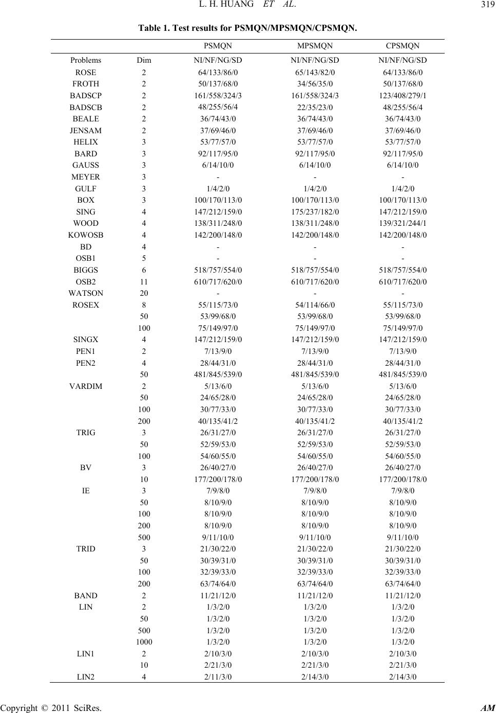

L. H. HUANG ET AL. 319
Table 1. Test results for PSMQN/MPSMQN/CPSMQN.
PSMQN MPSMQN CPSMQN
Problems Dim NI/NF/NG/SD NI/NF/NG/SD NI/NF/NG/SD
ROSE
FROTH
BADSCP
BADSCB
BEALE
JENSAM
HELIX
BARD
GAUSS
MEYER
GULF
BOX
SING
WOOD
KOWOSB
BD
OSB1
BIGGS
OSB2
WATSON
ROSEX
SINGX
PEN1
PEN2
VARDIM
TRIG
BV
IE
TRID
BAND
LIN
LIN1
LIN2
2
2
2
2
2
2
3
3
3
3
3
3
4
4
4
4
5
6
11
20
8
50
100
4
2
4
50
2
50
100
200
3
50
100
3
10
3
50
100
200
500
3
50
100
200
2
2
50
500
1000
2
10
4
64/133/86/0
50/137/68/0
161/558/324/3
48/255/56/4
36/74/43/0
37/69/46/0
53/77/57/0
92/117/95/0
6/14/10/0
-
1/4/2/0
100/170/113/0
147/212/159/0
138/311/248/0
142/200/148/0
-
-
518/757/554/0
610/717/620/0
-
55/115/73/0
53/99/68/0
75/149/97/0
147/212/159/0
7/13/9/0
28/44/31/0
481/845/539/0
5/13/6/0
24/65/28/0
30/77/33/0
40/135/41/2
26/31/27/0
52/59/53/0
54/60/55/0
26/40/27/0
177/200/178/0
7/9/8/0
8/10/9/0
8/10/9/0
8/10/9/0
9/11/10/0
21/30/22/0
30/39/31/0
32/39/33/0
63/74/64/0
11/21/12/0
1/3/2/0
1/3/2/0
1/3/2/0
1/3/2/0
2/10/3/0
2/21/3/0
2/11/3/0
65/143/82/0
34/56/35/0
161/558/324/3
22/35/23/0
36/74/43/0
37/69/46/0
53/77/57/0
92/117/95/0
6/14/10/0
-
1/4/2/0
100/170/113/0
175/237/182/0
138/311/248/0
142/200/148/0
-
-
518/757/554/0
610/717/620/0
-
54/114/66/0
53/99/68/0
75/149/97/0
147/212/159/0
7/13/9/0
28/44/31/0
481/845/539/0
5/13/6/0
24/65/28/0
30/77/33/0
40/135/41/2
26/31/27/0
52/59/53/0
54/60/55/0
26/40/27/0
177/200/178/0
7/9/8/0
8/10/9/0
8/10/9/0
8/10/9/0
9/11/10/0
21/30/22/0
30/39/31/0
32/39/33/0
63/74/64/0
11/21/12/0
1/3/2/0
1/3/2/0
1/3/2/0
1/3/2/0
2/10/3/0
2/21/3/0
2/14/3/0
64/133/86/0
50/137/68/0
123/408/279/1
48/255/56/4
36/74/43/0
37/69/46/0
53/77/57/0
92/117/95/0
6/14/10/0
-
1/4/2/0
100/170/113/0
147/212/159/0
139/321/244/1
142/200/148/0
-
-
518/757/554/0
610/717/620/0
-
55/115/73/0
53/99/68/0
75/149/97/0
147/212/159/0
7/13/9/0
28/44/31/0
481/845/539/0
5/13/6/0
24/65/28/0
30/77/33/0
40/135/41/2
26/31/27/0
52/59/53/0
54/60/55/0
26/40/27/0
177/200/178/0
7/9/8/0
8/10/9/0
8/10/9/0
8/10/9/0
9/11/10/0
21/30/22/0
30/39/31/0
32/39/33/0
63/74/64/0
11/21/12/0
1/3/2/0
1/3/2/0
1/3/2/0
1/3/2/0
2/10/3/0
2/21/3/0
2/14/3/0

L. H. HUANG ET AL. 320
Table 2. Relative efficiency of PSMQN, MPSMQN and
CPSMQN.
PSMQN MPSMQN CPSMQN
1 0.9752 0.9963
The geometric mean of these ratios for method EM(j)
over all the test problems is defined by




1S
i
iS
rEM jrEM j




, (4.3)
where S denotes the set of the test problems and S
the number of elements in S. One advan t ag e of the abo-
ve rule is that, the comparison is relative and hence does
not be dominated by a few problems for which the me-
thod requires a great deal of function evaluations and
gradient fu nct ions.
From Table 2, we observe that the average perfor-
mances of the Algorithm 1 are the best among the three
methods, and the average performances of the Algorithm
2 are little better than the PSMQN method. Therefore,
the Algorithm 1 is the best method among the three me-
thods given in this paper from both theory and the com-
putational point of view.
5. References
[1] J. M. Perry, “A Class of Conjugate Algorithms with a
Two Step Variable Metric Memory,” Discussion paper
269, Northwestern University, 1977.
[2] D. F. Shanno, “On the Convergence of a New Conjugate
Gradient Algorithm,” SIAM Journal on Numerical Anal-
ysis, Vol. 15, No. 6, 1978, pp. 1247-1257.
doi:10.1137/0715085
[3] J. Y. Han, G. H. Liu and H. X. Yin, “Convergence of
Perry and Shanno’s Memoryless Quasi-Newton Method
of Nonconvex Optimization Problems,” On Transactions,
Vol. 1, No. 3, 1997, pp. 22-28.
[4] J. J. More, B. S. Garbow and K. E. Hillstrome, “Testing
Unconstrained Optimization Software,” ACM Transac-
tions on Mathematical Software, Vol. 7, No. 1, 1981, pp.
17-41. doi:10.1145/355934.355936
[5] A. Griewank, “On Automatic Differentiation,” Kluwer
Academic Publishers, Norwell, 1989.
[6] Y. Dai and Q. Ni, “Testing Different Conjugate Gradient
Methods for Large-Scale Unconstrained Optimization,”
Journal of Computational Mathematics, Vol. 21, No. 3,
2003, pp. 311-320.