Applied Mathematics, 2011, 2, 303-308
doi:10.4236/am.2011.23035 Published Online March 2011 (http://www.scirp.org/journal/am)
Three New Hybrid Conjugate Gradient Methods
for Optimization*
Anwa Zhou, Zhibin Zhu, Hao Fan, Qian Qing
School of Mathematics and Computational Science, Guilin University of Electronic Technology,
Guilin, China
Received November 10, 2010; revised January 9, 2011; accepted January 14, 2011
Abstract
In this paper, three new hybrid nonlinear conjugate gradient methods are presented, which produce sufficient
descent search direction at every iteration. This property is independent of any line search or the convexity of
the objective function used. Under suitable conditions, we prove that the proposed methods converge glo-
bally for general nonconvex functions. The numerical results show that all these three new hybrid methods
are efficient for the given test problems.
Keywords: Conjugate Gradient Method, Descent Direction, Global Convergence
1. Introduction
In this paper, we consider the unconstrained optimizatio n
problem:

min, n
f
xxR (1.1)
where :n
f
RR is continuously differentiable and
the gradient of
f
at
x
is denoted by

g
x.
Due to its simplicity and its very low memory re-
quirement, the conjugate gradient (CG) method plays a
very important role for solving (1.1). Especially, when
the scale is large, the CG method is very efficient. Let
0n
x
R be the initial guess of the solution of problem
(1.1). A nonlinear conjugate gradient method is usually
designed by the iterative fo rm
1,0,1,, kkkk
xx dk

  (1.2)
where k
x
is the current iterate point, 0
k

 is a step-
length which is determined by some line search, and k
d
is the search direction defined by
1
,if0,
,if 0,
k
kkkk
gk
dgd k




 
 (1.3)
where k
g
denotes

k
g
x, and k

is a scalar. There
are some well-known formulas for k

, which are given
as follows:
2
2
1
,
k FR
k
k
g
g


 [1];
2
11
,
k CD
kT
kk
g
dg


 [2];
2
11
,
k DY
kT
kk
g
dy


 [3];
1
11
,
T
HS kk
kT
kk
gy
dy



 [4];
1
2
1
,
T
PRP kk
k
k
gy
g



 [5,6];
1
11
,
T
LS kk
kT
kk
gy
dg



 [7];
where 11kkk ygg



 and  stands for the Eucli-
dean norm of vectors.
Although the methods above are equivalent [8,9] when
f
is a strictly convex quadratic function and k

is
calculated by the exact line search, their behaviors for
general objective functions may be far different. Gener-
ally, in the convergence analysis of conjugate gradient
methods, one hopes the inexact line search such as the
Wolfe conditions, the strong Wolfe conditions or the
strong *Wolfe conditions,which are showed respectively
as follows:
1) The Wolfe line search is to find k

such that
*This work was supported in part by the NNSF (No. 11061011) o
f
China and Program for Excellent Talents in Guangxi Higher Education
Institutions ([2009]156).

A. W. ZHOU ET AL. 304


,
,
T
kkkk kkk
TT
kkkk kk
f
xdfx gd
dgx ddg


 




(1.4)
with 1
0,
2
  and 1.

 
2) The strong Wolfe line search is to findk

such that




,
,
T
kkkk kkk
TT
kkkk kk
f
xdfx gd
dgx ddg


 




(1.5)
with 1
0,
2
  and 1.

 
3) The strong *Wolfe line search is to find k

such
that




,
0,
T
kkkk kkk
TT
kkkk kk
f
xdfx gd
dg dgxd


 




(1.6)
with 1
0,
2
  and 1.

 
For general functions, Zoutendjk [10] and Al-Baali
[11] had proved the global convergence of the FR me-
thod with differen t lin e sear ches. And Powell [12] gave a
counter example which showed that there exist noncon-
vex functions such that the PRP method may cycle and
does not approach any stationary point even with exact
line search.Although one would be satisfied with its
global convergence, the FR method performs much
worse than the PRP (HS, LS) method in real computa-
tions. In other words, in practical computation, the PRP
method, the HS method, and the LS method are generally
believed to be the most efficient conjugate gradient me-
thods since these methods essentially perform a restart if
a bad direction occurs. A similar case happens to the DY
method and the CD method. That is to say the conver-
gences of the CD , DY and FR methods are established
[1-3], however their numerical results are not so well.
Resently, some good results on the nonlinear conjugate
gradient method are given. Combining the good numeri-
cal performance of the PRP and HS methods and the nice
global convergence properties of the FR and DY me-
thods, recently, [13] and [14] proposed some hybrid me-
thods which we call the H1 method and the H2 method,
respectively, that is,
 
1max 0,min,, HPRP FR
kkk
  (1.7)


2max 0,min,. HHSDY
kkk
  (1.8)
Gilbert and Nocedal [15] extended H1 to the case that
 
max,min ,.
FRPRP FR
kkkk
 
Numerical performances show that the H1 and the H2
methods are better than the PRP method [13,14,16].
As we all know, the FR , DY and CD methods are
descent methods, but their descent properties depend on
the line se arch su ch as the strong Wo lfe line se arch (1 .5).
Similar to the descent three terms PRP method in [17],
Zhang et al. [18,19] proposed a modified FR method
which we call the MFR method, that is,
1
1
11
11
2
:
1.
T
FR kk
kkkk k
T
kk
T
FR FR kk
kkkk
k
gd
MFR dgdg
dg
gd
g
d
g







 


 


(1.9)
And [18] also gave an equivalent form to the MFR
method. Similarly, Zhang [19] also proposed a modified
DY method called the MDY method, that is,
DY 1
1
11
DY DY
11
2
DY :
1
T
kk
kkkk k
T
kk
T
kk
kkkk
k
gd
Mdg dg
dg
gd
g
d
g







 


 


(1.10)
It is easy to see that the MFR and MDY methods have
an important property that the search directions satisfy
2,
T
kk k
gd g which depend s neither on the line search
used nor on the convexity of the objective function;
moreover these two methods reduce to the FR method
and the DY method respectively with exact line search.
[18] has explored the convergence and efficiency of
the MFR method for nonconvex functions with the
Wolfe line search or Armijo line search. Based on the
idea of the H1 and the H2 methods, recently, Zhang-
Zhou [20] replaced
F
R
k

in (1.9) and DY
k

in (1.10)
with H1
k

in (1.7) andH2
k

in (1.8), respectively, and
proposed two new hybrid PRP–FR and HS–DY methods
called the NH1 method and the NH2 method, respec-
tively, that is,
H1 H1 11
2
N1:1 T
kk
kk kkk
k
gd
H
dgd
g





 


(1.11)
H2 H2 11
2
N2:1 T
kk
kk kkk
k
gd
H
dgd
g




  


(1.12)
Obviously, these two new hybrid methods still satisfy
2,
T
kk k
gd g (1.13)
which shows that they are descent and independent of
any line search used. [20] proved the global convergence
of these two methods and also showed their efficiency in
real computations.
Similarly,based on the idea of the methods all above,
we consider the CD method, and propose three new hy-

A. W. ZHOU ET AL. 305
brid conjugate gradient(CG) methods which we call the
H3 method, the MCD method and the NH3 method, re-
spectively, that is

 
3
3:max 0,min,
HLSCD
kkk
H   (1.14)
1
1
11
11
2
:
1
T
CD kk
kkkkk
T
kk
T
CD CD kk
kkkk
k
gd
MCD dgdg
dg
gd
g
d
g







 


 


(1.15)
H3 H3 11
2
N3:1 T
kk
kk kkk
k
gd
H
dgd
g




  


(1.16)
From these three methods above, it is not difficult to
see that the MCD and the NH3 methods also sat-
isfy 2,
T
kk k
gd g which shows that they are suffi-
cient descent methods. In the next section, the new algo-
rithms are given. The global convergence of the pro-
posed methods are proved in Section 3. We give the nu-
merical experiments in Section 4, and in Section 5, the
conclusion is presented.
2. Algorithm
2.1. Algorithm 1 (The H3 Algorithm)
Step 0: Choose an initial point 0,
n
x
R01,


1
0,
2
  and 1.

  Set 00 ,:0.dgk
Step 1: If ,
k
g

then stop; Otherwise go to the next
step.
Step 2: Compute step size k

by strong *Wolfe line
search rule (1.6).
Step 3: Let 1.
kkkk
x
xd

 If 1, k
g

 then stop.
Step 4: Calculate the search direction
3
111
.
H
kkkk
dg d 

 
Step 5: Set :1,kkand go to Step 2.
2.2. Algorithm 2 (The MCD (Or the NH3)
Algorithm)
Step 0: Choose an initial point 0,
n
x
R01,


1
0,
2
  and 1.

  Set 00 ,:0.dgk
Step 1: If ,
k
g

then stop; otherwise go to the next
step.
Step 2: Compute step size k

by Wolfe line search
rule (1.4).
Step 3: Let 1.
kkkk
x
xd



 If 1,
k
g

, then stop.
Step 4: Calculate the search direction 1k
d by (1.15)
(or (1.16)).
Step 5: Set :1,kk

 and go to Step 2.
3. The Global Convergence
Assumption A
1) The level set
 


0
n
x
Rfx fx is bounded,
where 0,
n
x
Ris a given point.
2) In an open convex set N that contains

,
f
is
continuously differentiable and its gradient
g
is Lipschitz
continuous, namely, there exists a constant 0L such
that




,, .
g
xgyLxyxyN
(3.1)
Since




k
f
xis decreasing, it is clear that the se-
quence


k
x
generated by Algorithm 1 and Algorithm 2 is
contained in

. In addition, we can get from Assump-
tion A that there exists a constant B and 10,

such that


1
,,.xBgx x 

 (3.2)
In the latter part of the paper, we always suppose that
the conditions in Assumption A hold. Then there is an
useful lemma, which was originally given in [10,21].
Lemma 3.1 Let


k
x
be generated by (1.2) andk dis a
descent direction. If k

is determined by the Wolfe line
search (1.4), then we have

2
2
0.
T
kk
kk
gd
d



 (3.3)
From Lemma 3.1 and (1.13) that for the MCD and
NH3 methods with the Wolfe line search,we can easily
obtain the following condition
4
2
0.
k
kk
g
d



 (3.4)
We now establish the global convergence theorem for
Algorithm 1 and Algorithm 2 .
3.1. The Global Convergence of the H3 Method
For simlpicity, here, we list the Theorem 2.3 in [14] as
the following Lemma 3.2 without proof.
Lemma 3.2 Suppose that 0
x
is an initial point, Con-
sider the method (1.2) and (1.3), where k

is computed
by the Wolfe line search(1.4), andk

is such that


,1 ,
k
rc where 1
,0.
1
k
kDY
k
rc


 




Then if 0
k
g

for all 0,kwe have that

A. W. ZHOU ET AL. 306
0, 0.
T
kk
gd k
Further, the method converges in the sense that
liminf 0.
k
kg  
From the Lemma 3.2 above, similar to Corollary 2.4 in
[14], we give the global convergence of the H3 me-
thod(Algorithm 1).
Theorem 3.3 Suppose that0 xis an initial point, Con-
sider the Algorithm1, then we have either0
k
g

for
some 0,k or liminf 0.
k
kg


Proof From the second inequality of (1.6) and the de-
finitions of 3,
H
CD
kk

 and ,
D
Y
k
 it follows that
3
0.
H
CD DY
kkk
 
Therefore the statement follows lemma 3.2. 
3.2. The Global Convergence of the MCD
Method
Now, we establish the global convergence theorem for
the MCD method.
Theorem 3.4 Let

k
x
be generated by the MCD me-
thod (Algorithm 2, wherek
d satisfies (1.15)), then we
have liminf 0.
k
kg
  (3.5)
Proof Suppose by contradiction that the desired con-
clusion is not true, that is to say, there exists a con-
stant 0

such that
,0.
k
gk   (3.6)
Set 1
2
1,
T
CD kk
kk
k
gd
hg 

 and then we have
22
1.
CDT
kkk kkk
gdh gg 
From (1.15) and (1.13), it
follows that




2
2
1
222
2
11
2222 2
2
11
2222
2
1
2
2
2
CD
kkkkk
CDCD T
kk kkkkkk
CD T
kk kkkkkkkk
CD
kk kkkk
ddhg
dhdghg
dhhggdghg
dhghg













222
2
12
CD T
kk kkkkk
dhdghg 

 (3.7)
Dividing both sides of (3.7) by

2
T
kk
g
d, we get, from
(1.13) and the definition ofCD
k

, that

22
42
kk
T
kkk
dd
ggd






22
2
21
22
22 2
2
1 2
22 2
1
2
12
42
1
2 2
1
422
1
2
1
42
1
22
0
2
2
()
1211
11
1
1.
kkk
CD k
kT
TT
kk
kk kk
kk kk
k
T
TT
kk
kkk kk
kkk
kk
kk
kkk
k
kk
k
ii
dhg
h
gd
gd gd
gd hg
h
gd
ggd gd
dhh
gg
hd
ggg
d
gg
k
g














 

 



The last inequality implies
4
2
2
00
1,
k
kk
k
g
k
d





which contradicts (3.4). The proof is then completed. 
3.3. The Global Convergence of the NH3
Method
The same as the Theorem 3.4, we can establish the fol-
lowing global convergence theorem for the NH3 method.
Theorem 3.5 Let


k
x
be generated by the NH3 me-
thod (Algorithm 2, where k d satisfies (1.16) ), then we
have
liminf 0.
k
xg   (3.8)
Proof Suppose by contradiction that the desired con-
clusion is false, that is to say, there exists a con-
stant 0

such that
,0.
k
gk   (3.9)
Similar to (3.7), we get from (1.16) that

2
22 2
32
12,
HT
kkk kkkkk
ddhdghg 


(3.10)
where
31
2
1.
T
Hkk
kk
k
gd
hg 


Notice that
3,0.
HCD
kk
k 

 (3.11)
Dividing both sides of (3.10) by

2
T
kk
g
d, we get,
from (3.11), (1.13) and the definition of 3,
H
k
 that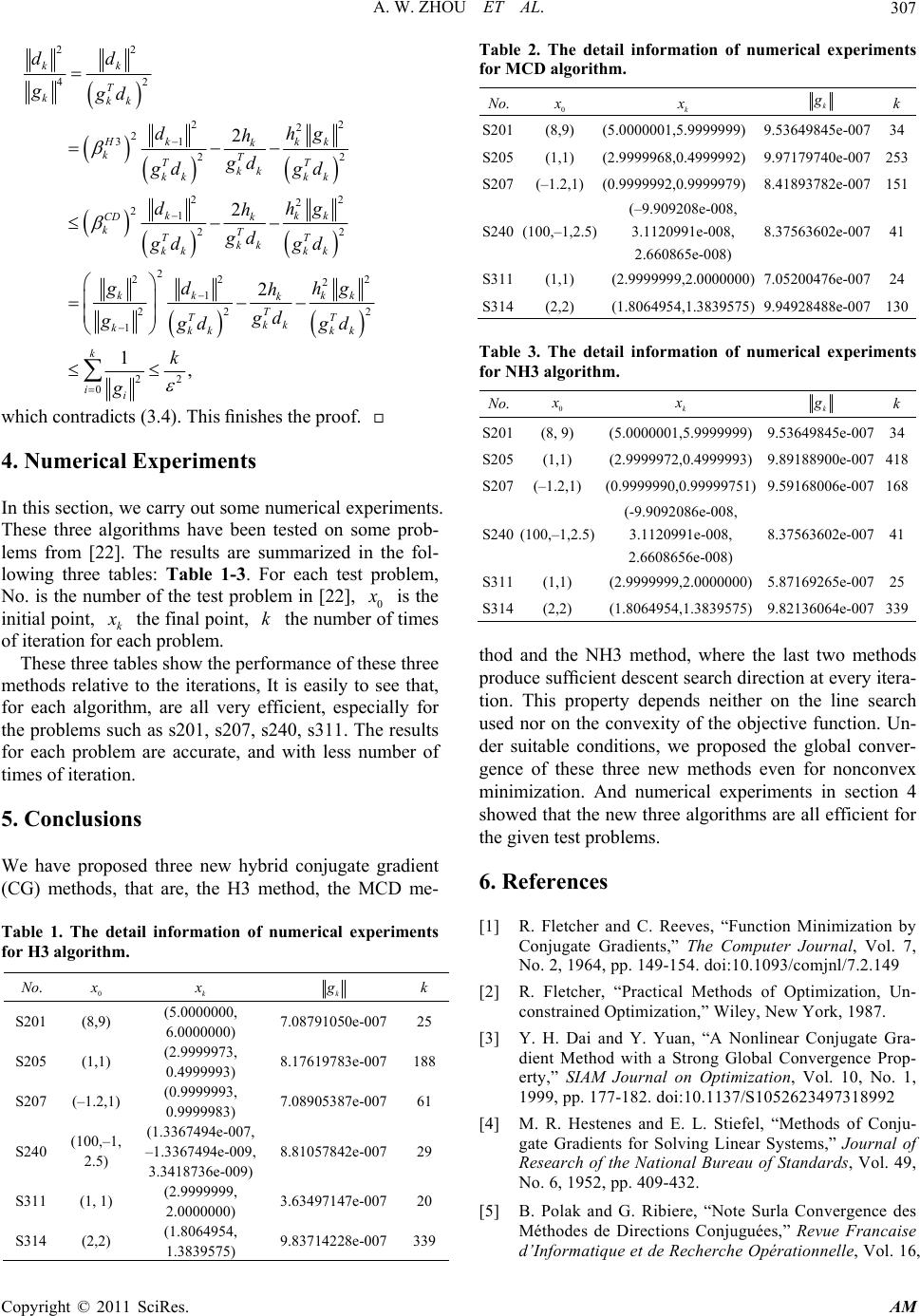

A. W. ZHOU ET AL. 307

22
42
kk
T
kkk
dd
ggd


 

 

22
2
21
3
22
22
2
21
22
2
22 2
2
1
22 2
1
22
0
2
2
2
1,
kkk
Hk
kT
TT
kk
kk kk
kkk CD k
kT
TT
kk
kk kk
kk kk
k
T
TT
kk
kkk kk
k
ii
dhg
h
gd
gd gd
dhg
h
gd
gd gd
gd hg
h
gd
ggd gd
k
g











 




which contradicts (3.4). This finishes the proof. 
4. Numerical Experiments
In this section, we carry out some numerical experiments.
These three algorithms have been tested on some prob-
lems from [22]. The results are summarized in the fol-
lowing three tables: Table 1-3. For each test problem,
No. is the number of the test problem in [22], 0
x
is the
initial point, k
x
the final point, k the number of times
of iteration for each problem.
These three tables show the performance of these three
methods relative to the iterations, It is easily to see that,
for each algorithm, are all very efficient, especially for
the problems such as s201, s207, s240, s311 . The results
for each problem are accurate, and with less number of
times of iteration.
5. Conclusions
We have proposed three new hybrid conjugate gradient
(CG) methods, that are, the H3 method, the MCD me-
Table 1. The detail information of numerical experiments
for H3 algorithm.
.No 0
x
k
x
k
g
k
S201 (8,9) (5.0000000,
6.0000000) 7.08791050e-00725
S205 (1,1) (2.9999973,
0.4999993) 8.17619783e-007 188
S207 (–1.2,1) (0.9999993,
0.9999983) 7.08905387e-00761
S240 (100,–1,
2.5)
(1.3367494e-007,
–1.3367494e-009,
3.3418736e-009) 8.81057842e-00729
S311 (1, 1) (2.9999999,
2.0000000) 3.63497147e-00720
S314 (2,2) (1.8064954,
1.3839575) 9.83714228e-007 339
Table 2. The detail information of numerical experiments
for MCD algorithm.
.No 0
x
k
x
k
g
k
S201(8,9) (5.0000001,5.9999999) 9.53649845e-00734
S205(1,1) (2.9999968,0.4999992) 9.97179740e-007253
S207(–1.2,1) (0.9999992,0.9999979) 8.41893782e-007 151
S240 (100,–1,2.5)
(–9.909208e-008,
3.1120991e-008,
2.660865e-008)
8.37563602e-007 41
S311(1,1) (2.9999999,2.0000000) 7.05200476e-00724
S314(2,2) (1.8064954,1.3839575) 9.94928488e-007130
Table 3. The detail information of numerical experiments
for NH3 algorithm.
.No 0
x
k
x
k
g
k
S201(8, 9) (5.0000001,5.9999999) 9.53649845e-00734
S205(1,1) (2.9999972,0.4999993) 9.89188900e-007418
S207(–1.2,1) (0.9999990,0.99999751) 9.59168006e-007168
S240 (100,–1,2.5)
(-9.9092086e-008,
3.1120991e-008,
2.6608656e-008)
8.37563602e-007 41
S311(1,1) (2.9999999,2.0000000) 5.87169265e-00725
S314(2,2) (1.8064954,1.3839575) 9.82136064e-007339
thod and the NH3 method, where the last two methods
produce sufficient descent search direction at every itera-
tion. This property depends neither on the line search
used nor on the convexity of the objective function. Un-
der suitable conditions, we proposed the global conver-
gence of these three new methods even for nonconvex
minimization. And numerical experiments in section 4
showed that the new three algorithms are all efficient for
the given test problems.
6. References
[1] R. Fletcher and C. Reeves, “Function Minimization by
Conjugate Gradients,” The Computer Journal, Vol. 7,
No. 2, 1964, pp. 149-154. doi:10.1093/comjnl/7.2.149
[2] R. Fletcher, “Practical Methods of Optimization, Un-
constrained Optimization,” Wiley, New York, 1987.
[3] Y. H. Dai and Y. Yuan, “A Nonlinear Conjugate Gra-
dient Method with a Strong Global Convergence Prop-
erty,” SIAM Journal on Optimization, Vol. 10, No. 1,
1999, pp. 177-182. doi:10.1137/S1052623497318992
[4] M. R. Hestenes and E. L. Stiefel, “Methods of Conju-
gate Gradients for Solving Linear Systems,” Journal of
Research of the National Bureau of Standards, Vol. 49,
No. 6, 1952, pp. 409-432.
[5] B. Polak and G. Ribiere, “Note Surla Convergence des
Méthodes de Directions Conjuguées,” Revue Francaise
d’Informatique et de Recherche Opérationnelle, Vol. 16,

A. W. ZHOU ET AL. 308
No. 1, 1969, pp. 35-43.
[6] B. T. Polyak, “The Conjugate Gradient Method in Ex-
treme Problems,” USSR Computational Mathematics
and Mathematical Physics, Vol. 9, No. 4, 1969, pp.
94-112. doi:10.1016/0041-5553(69)90035-4
[7] Y. L. Liu and C. S. Storey, “Efficient Generalized Con-
jugate Gradient Algorithms, Part 1: Theory,” Journal of
Optimization Theory and Applications, Vol. 69, No. 1,
1991, pp. 129-137. doi:10.1007/BF00940464
[8] Y. Yuan and W. Sun, “Theory and Methods of Optimi-
zation,” Science Press of China, Beijing, 1999.
[9] Y. H. Dai and Y. Yuan, “Nonlinear Conjugate Gradient
Methods,” Shanghai Scientific and Technical Publishers,
Shanghai, 1998.
[10] G. Zoutendijk, “Nonlinear Programming, Computation-
al Methods,” In: J. Abadie Ed., Integer and Nonlinear
Programming, North-Holland, Amsterdam, 1970, pp.
37-86.
[11] M. Al-Baali, “Descent Property and Global Conver-
gence of the Fletcher–Reeves Method with Inexact Line
Search,” IMA Journal of Numerical Analysis, Vol. 5, No.
1, 1985, pp.121-124. doi:10.1093/imanum/5.1.121
[12] M. J. D. Powell, “Nonconvex Minimization Calcula-
tions and the Conjugate Gradient Method,” Lecture
Notes in Mathematics, Vol. 1066, No. 122, 1984, pp.
121-141.
[13] D. Touati-Ahmed and C. Storey, “Efficient Hybrid
Conjugate Gradient Techniques,” Journal of Optimiza-
tion Theory and Applications, Vol. 64, No. 2, 1990, pp.
379–397. doi:10.1007/BF00939455
[14] Y. H. Dai and Y. Yuan, “An Efficie nt Hybrid Con jugate
Gradient Method for Unconstrained Optimization,”
Annals of Operatio ns Research, Vol. 103, No. 1-4, 2001,
pp. 33-47. doi:10.1023/A:1012930416777
[15] J. C. Gilbert and J. Nocedal, “Global Convergence
Properties of Conjugate Gradient Methods for Optimi-
zation,” SIAM Journal Optimization, Vol. 2, No. 1,
1992, pp. 21-42. doi:10.1137/0802003
[16] W. W. Hager and H. Zhang, “A New Conjugate Gra-
dient Method with Guaranteed Descent and an Efficient
Line Search,” SIAM Journal Optimization, Vol. 16, No.
1, 2005, pp. 170-192. doi:10.1137/030601880
[17] L. Zhang, W. J. Zhou and D. H. Li, “A Descent Mod-
ified Polak-Ribière-Polyak Conjugate Gradient Method
and Its Global Convergence,” IMA Journal of Numeri-
cal Analysis, Vol. 26, No. 4, 2006, pp. 629-640.
doi:10.1093/imanum/drl016
[18] L. Zhang, W. J. Zhou and D. H. Li, “Global Conver-
gence of a Modified Fletcher-Reeves Conjugate Method
with Armijo-Type Line Search,” Numerische Mathema-
tik, Vol. 104, No. 4, 2006, pp. 561-572.
doi:10.1007/s00211-006-0028-z
[19] L. Zhang, “Nonlinear Conjugate Gradient Methods for
Optimization Problems,” Ph.D. Thesis, Hunan Univer-
sity, 2006.
[20] L. Zhang and W. J. Zhou, “Two Descent Hybrid Con-
jugate Gradient Methods for Optimization,” Journal of
Computati onal and Applied Mat hematics, Vol. 216, No.
1, 2008, pp. 251-264. doi:10.1016/j.cam.2007.04.028
[21] P. Wolfe, “Convergence Conditions for Ascent Me-
thods,” SIAM Review, Vol. 11, No. 2, 1969, pp. 226-235.
doi:10.1137/1011036
[22] W. Hock and K. Schittkowski, “Test Examples for Non-
linear Programming Codes,” Journal of Optimization
Theory and Applications, Vol. 30, No. 1, 1981, pp.
127-129. doi:10.1007/BF00934594