 Journal of Computer and Communications, 2014, 2, 172-181 Published Online March 2014 in SciRes. http://www.scirp.org/journal/jcc http://dx.doi.org/10.4236/jcc.2014.24023 How to cite this paper: Wu, S.-F., Chiou, Y.-S. and Lee, S.-J. (2014) Multi-Valued Neuron with Sigmoid Activation Function for Pattern Classification. Journal of Computer and Communications, 2, 172-181. http://dx.doi.org/10.4236/jcc.2014.24023 Multi-Valued Neuron with Sigmoid Activation Function for Pattern Classification Shen-Fu Wu, Yu-Shu Chiou, Shie-Jue Lee Department of Electrical Engineering, National Sun Yat-sen University Email: sfwu@water.ee.nsysu.edu.tw, yschiou@water.ee.nsysu.edu.tw, leesj@mail.ee.nsysu.edu.tw Received December 2013 Abstract Multi-Valued Neuron (MVN) was proposed for pattern classification. It operates with complex-va- lued inputs, outputs, and weights, and its learning algorithm is based on error-correcting rule. The activation function of MVN is not differentiable. Therefore, we can not apply backpropagation when constructing multilayer structures. In this paper, we propose a new neuron model, MVN-sig, to simulate the mechanism of MVN with differentiable activation function. We expect MVN-sig to achieve higher performance than MVN. We run several classification benchmark datasets to com- pare the performance of MVN-sig with that of MVN. The experimental results show a good poten- tial to develop a multilayer networks based on MVN-sig. Keywords Pattern Classification; Mu lt i -Valued Neuron (MVN); Differentiable Activation Function; Backpropagation 1. Introduction The discrete multi-valued neuron (MVN) was proposed by N. Aizenberg and I. Aizenberg in [1] for pattern classification. The neuron operates with complex-valued inputs, outputs, and weights. Its inputs and outputs are mapped onto the complex plane. They are located on the unit circle, and are exactly the roots of unity. The activation function of MVN -valued logic maps a set of the roots of unity on itself. Two discrete-valued MVN learning algorithms are presented in [2]. They are based on error-correcting learning rule and are deriva- tive-free. This makes MVN have higher functionality than sigmoidal or radial basis function neurons. The multilayer feedforward neural network based on MVN (MLMVN) was introduced in [3,4]. This model can achieve good performance using simpler structures. MLMVN learning rule is heuristic error backpropa- gation due to the fact that the activation function of MVN is not differentiable. The error with certain neuron is retrieved from next layer and evenly shared among the neurons connected from the former layer and itself. We can not apply function optimization methods to this model because of the activation function. This property led us to develop a multi-valued neuron with a differentiable activation function. 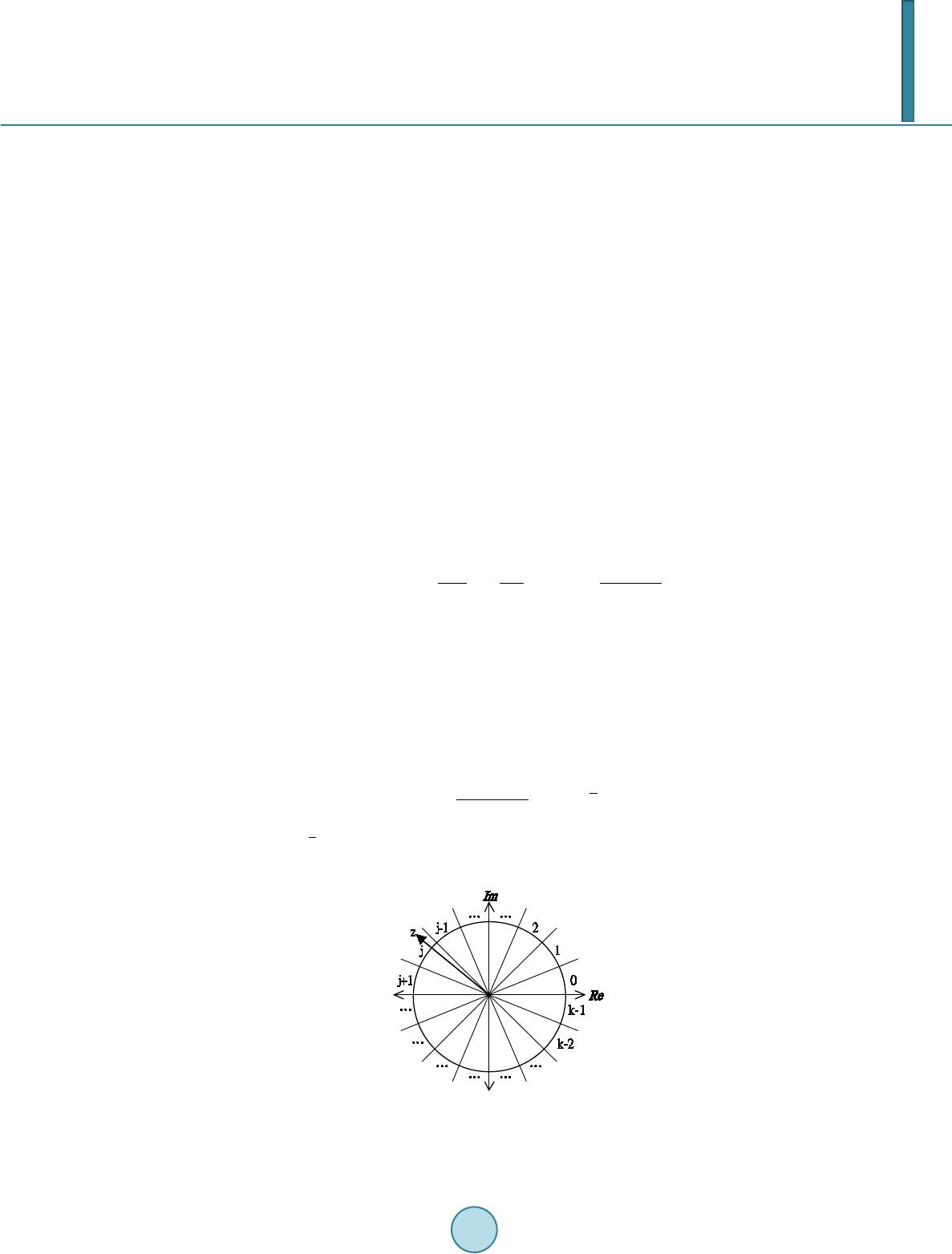 S.-F. Wu et al. In this paper, we propose a new neuron model, MVN-sig, to simulate the mechanism of MVN with dif- ferentiable activation function. We consider the activation function of MVN as a function of the argument of a weighted sum. We stack multiple sigmoid functions to approximate this multiple step function. Hence, we can obtain a differentiable input/output mapping and we apply a naive gradient descent method as its learning rule. We expect MVN-sig to achieve better performance than MVN. The rest of the paper is organized as follows. Section 2 briefly describes MVN and its activation function. Section 3 presents MVN-sig and the sigmoid activation function. The learning algorithm of MVN-sig is des- cribed in detail. Section 4 presents the results of three experiments. Finally, conclusions and discussions are given in Section 5. 2. Multi-Valued Neuron 2.1. Discrete MVN A discrete-valued MVN is a function mapping from a -feature input onto a single output. This mapping is described by a multiple-valued ( -valued) function of -feature instances, , which uses complex-valued weights: )(=),,( 1101 nnn xxPxxf ωωω +++ (1) where , are the features of an instance, on which the performed function depends, and , , are the weights. The values of the function and of the features are complex. They are the roots of unity: , , and is an imaginary unity. is the activation function of the neuron: k j zarg k j if k ji zP1)(2 <)( 2 ), 2 (exp=)( + ≤ πππ (2) where are values of the -valued logic, is the weighted sum, and is the argument of the complex number . Equation (2) is illustrated in Figure 1. Equation (2) divides the complex plane into equal sectors and maps the whole complex plane onto a subset of points belonging to the unit circle. This subset corresponds exactly to a set of the roots of unity. The MVN learning is reduced to the movement along the unit circle and is derivative-free. The movement is determined by the error which is the difference between the desired and actual output. The error-correcting learning rule and the corresponding learning algorithm for the discrete-valued MVN were described in [5 ] and modified by I. Aizenberg and C. Moraga [3]: ,)( ||1)( = 1i sq r r r i r i x zn C ε εωω − + + + (3 ) for , where is the input of feature with the components complex-conjugated, is the number of the input features, is the desired output of the neuron, is the actual output of the Figure 1. Geometrical interpretation of the discrete-valued MVN activation function.  S.-F. Wu et al. neuron (see Figure 2), is the number of the learning epoch, is the current weighting of the feature, is the following weighting of the feature after correction, is the constant part of the learning rate (it may always equal to 1), and is the absolute value of the weighted sum obtained on the epoch. The factor is useful when learning non-linear functions with a number of high irregular jumps. Equation (3) ensures that the corrected weighted sum moves from sector to sector (see Figure 2(a)). The direction of this movement is determined by the error . The convergence of the learning algorithm was proven in [6]. 2.2. Continuous MVN The activation function Equation (2) is piece-wise discontinuous. This function can be modified and generalized for the continuous case in the following way. When in Equation (2), the angle value of the sector (see in Figure 1) will approach to zero. The activation function is transformed as follows: (4) where is the weighted sum, is the argument of complex number , and is the modulus of the complex number . The activation function Equation (4) maps the weighted sum into the whole unit circle (see Figure 2(b)). Equation (2) maps only to the discrete subsets of the points belonging to the unit circle. Equation (2) and Equation (4) are both not differentiable, but their differentiability is not required for MVN learning. The Learning rule of the continuous-valued MVN is shown as follows: 1 =()=(), (1) ||(1) |||| rrqsrq rr i iiii rr CC z xx nznz z ωωεεωε + +−+− ++ (5) for . 3. MVN with Sigmoid Activation Function The learning algorithm of MVN is reduced to the movement along the unit circle on the complex plane. They are based on error-correcting learning rule and are derivative-free. Therefore, we can not use chain rule for error backpropagation to construct multilayer networks using MVN. In [3], I. Aizenberg and C. Moraga introduced a heuristic approach to construct the multilayer feedforward neural networks based on MVN. This inspired us to develop a differentiable activation function to which we can apply backpropagation learning rule. We expect the new learning rule to have more execution time but it can achieve better performance than MVN on a single neuron. (a) (b) Figure 2. Geometrical interpretation of the MVN learning rule: (a) Discrete- valued MVN; and (b) Continuous-valued MVN.  S.-F. Wu et al. 3.1. Multi-Valued Sigmoid Activation Function The basic idea of the multi-valued sigmoid activation function is to approximate the functionality of MVN using multiple sigmoid functions. In [7], E. Wilson presented a similar model for robot thruster control and farther applications. The original activation function of MVN is written in Equa tion (2). This activation function operates with the argument of weighted sum. Therefore, we can transfer this activation function into a function of argument which is illustrated in Figu re 3. The corresponding MVN presentation is in Figure 4. This form of original activation function of MVN is a combination of multiple step functions, which can be approximated by stacking multiple sigmoid functions: 1() 1 11 11 () 1 =1 =1 2/ ( )=1exp 2/ ( )=( )=1exp ici kk ici ii k f k Ff θτ θτ π θ π θθ −− −− −− + + ∑∑ (6) where is the multi-valued sigmoid activation function, is the argument of weighted sum, is the argument of root of unity and is the sigmoid function setting on . The activation function in Equation (6) is a mapping from the argument of weighted sum onto the argument of certain root of unity. Hence, we use Euler’s formula in Equation (7) to transfer the outcome to a complex value. (7) where is the outcome of activation function . We can approach the functionality of MVN activation function in Equation (2) by using Equations (6) and (7). Therefore, we can build a new model architecture which Figure 3. MVN activation function represents the set of roots of unity by their arguments. Figure 4. Geome trical interpretation of MVN activation function by .  S.-F. Wu et al. can not only solve multi-valued logic problems but also be differentiable. We call this model “MVN-sig” and its model architecture is illustrated in Figure 5. Since the activation function is no longer discrete-valued, we need to determine how to obtain the cor- responding label for classification problems. The most intuitive method is to equally divide the mapped range of the activation function. This label judgement method is illustrated in F i g ure 6. 3.2. Learning Single Neuron Using Gradient Descent Method Because the MVN-sig a complex-valued neuron, the output of MVN-sig can be derived from input: ,,, , = ,= jj rejimjj rejim xxxww w ++ (8) where and indicate the real and imaginary parts of input variable, respectively. Likewise, and indicate the real and imaginary parts of weight. Thus, the weighted sum of a given n-variable instance can be written as: ,, ,,,, ,, =0 =0=0 ==() () nn n jjj rej rej imj imj imj rej rej im jj j zwxwxwxi wxwx−+ + ∑∑ ∑ (9) Let the output of MVN-sig be 2 22 =)()(== ˆ θ θθ i ttt eisincosibay ++ . For an instance , and are the real and imaginary parts of MVN-sig output, respectively. 22 11 ˆ== ()()= (())(()) =(( ()))(( ())) ttt yaibcosisincos Fisin F cosF arg zisinF arg z θθ θθ ++ + + (10) Figure 5. MVN-sig model architecture. Figure 6. Label judgement.  S.-F. Wu et al. The error function for an instance is defined as: (1 1 ) where is the desired output and is the actual output of MVN-sig neuron. is the error between the desired value and the output. signifies the complex conjugate of . Let the desired output be . )()(= ˆ = ttttttt biayy −+−− βαδ . Hence, the error function is a real scalar function: })(){( 2 1 = 2 1 = 22ttttttt baE −+− βαδδ (12) In order to use the chain rule to find the gradient of error function , we have to calculate both real and imaginary parts independently. In Equation (12), we observe that is a function of both and , and and are both functions of and . We defined the gradient of the error func- tion with respect to the complex-valued weight as follows: ,, = ()=() def t tt jjj rej im E EE wi w ww ηη ∂ ∂∂ ∆−− + ∂ ∂∂ (13 ) The gradient of the error function with respect to the real and imaginary parts of can be written as: ,, , ( ())() =( ) ( ())() ( ())() () ( ())() tt t j retj re tt tj re EEa Farg zarg z waF argzarg zw Eb Farg zargz bF arg zarg zw ∂∂∂ ∂∂ ∂ ∂∂∂∂ ∂∂ ∂∂ +∂∂∂ ∂ (14) ,, , ( ())() =( ) ( ())() ( ())() () ( ())() tt t j imtjim tt tj im EEa Farg zarg z waFarg zarg zw Eb Farg zarg z bF arg zarg zw ∂∂∂ ∂∂ ∂ ∂∂∂∂ ∂∂ ∂∂ +∂∂∂ ∂ (15) We can combine Equation (14) and Equation (15) into Equation (13): ,, ={ } ( ())( ()) ( ())()() { }{} () tt tt jtt j rej im Ea Eb waF arg zbF arg z Farg zarg zarg z i arg zww η ∂∂ ∂∂ ∆− + ∂∂ ∂∂ ∂ ∂∂ + ∂ ∂∂ (16) Firstly, we derive each term within the first braces in Equation (16) from Equation (12) and Equatio n (10): (17) (18) )))(((= ))(( )))((( = ))(( zargFsin zargF zargFcos zargF at− ∂ ∂ ∂ ∂ (19) )))(((= ))(( ))) ((( = ))(( zargFcos zargF zargFsin zarg F b t ∂ ∂ ∂ ∂ (20) where and represent the real and imaginary parts of . Secondly, the second braces in  S.-F. Wu et al. Equation (16) contains the derivative of the multi-valued sigmoid activation function. We can derive this acti- vation function in Equation (6): (() ) 11 (() )(() ) =1 =1 (( ))2/2exp == ()() 11 exp exp c argz kk i c argzc argz ii ii F arg zkc arg zarg zk τ ττ ππ −− −− −− −− ∂∂ ∂∂++ ∑∑ ( 21 ) Finally, the third braces in Equation (16) contains the derivatives of the argument of weighted sum . The derivation is shown as follows: 122 ()()()()() () = ()= () () () jj argzIm zRe z ImzRez Im z tan wwRe zRe zIm z − ′′ ∂∂ − ∂∂ + (22) where and represent the real and imaginary parts of weighted sum and and represent their derivatives, respectively. From Equation (9), we can simplify this equation: ),(= )( ),(= )( ,, j rej j rej xIm w zIm xRe w zRe ∂ ∂ ∂ ∂ (23) )(= )( ),(= )( ,, j imj j imj xRe w zIm xIm w zRe ∂ ∂ − ∂ ∂ (24) where and represent the real and imaginary parts of input variable . Thus, the derivatives of the argument of weighted sum with respect to the real ( ) and imaginary parts is shown as follows: ))()()()(( || 1 = )( 2 ,jj rej xRezImxImzRe z w zarg − ∂ ∂ (25) ))()()()(( || 1 = )( 2 ,jj imj xImzImxRezRe z w zarg + ∂ ∂ (26) j imjrej x z z i w zar g i w zar g 2 ,, || = )()( ∂ ∂ + ∂ ∂ (27) where represents the complex conjugate of input variable . From Equations (17)-(21) and (27), we can generate the learning rule of input weighting : () 11 22 () 2 1 =1 2exp ={( )()( )( )}{}{} || 1exp c ki jt tj ci i cz wRe sinIm cosix kz θτ θτ π ηδ θδθ −− − −− ∆− −+ ∑ (28) where is the argument of the weighted sum and is the output of multi-valued sigmoid activation func- tion ( ). 3.3. Stopping Criteria We combine two stopping criteria to make sure the learning process stops when the output is accurate and stable. Firstly, we continue to iterate until the difference between the network response and the target function reaches some acceptable level. In Equation (29 ), we keep tracking the mean squared error until it reaches a given value . Secondly, we check the relative change in the training error is small using Equation (30). (29) Λ≤ − − − − )}()({ 2 1|)()(| 1 1 tt tt wEwE wEwE (30)  S.-F. Wu et al. where is the total number of learning instances, is the error between desired value and estimation, and and represent the mean squared errors at and learning epochs. Figure 7 shows two examples of error convergence. Vertical and horizontal axis represent mean squared error and time epoch, respectively. In Figure 7(a), if we only use Equation (30) as the stopping criterion, the learning process will stop early and has worse training and testing accuracy. On the other hand, if we do not use Equation (30), it will take too much time to converge. In Figure 7(b), we can see the learning process is relatively stable after 300 epochs. We monitored the testing accuracy at 300 epoch and at the end of learning process. They did not change much during this interval and that is why we use Equation (29) and Equation (30) as our stopping criteria. 3.4. MVN-Sig Learning Algorithm We develop the learning algorithm based on the multi-valued sigmoid function and the gradient descent method. The convergence of the learning algorithm can be proven based on the convergence of the gradient descent method in [8]. The implementation of the proposed learning algorithm in one iteration consists of the following steps: procedure MVN-sig This is one learning epoch with N learning instances Let represents the instance Let z be the current value of weighted sum. / Equation (10) / while do Check equation with activation function. for j = 0 to n do / -variable instance / / Equation (28) / end for n r n rr x wx w w z 1 1 1 1 1 0 = ~ + ++ ++ + end while Iterates until the outcome meets stopping criteria. / Equation (29) and Equation (30) / end procedure 4. Simulation Results The proposed strategies and learning algorithms are implemented and checked over a given three benchmark (a) (b) Figure 7. MSE-epoch plots.  S.-F. Wu et al. datasets [9]. The software simulator is written in Matlab R2011b (64-bit) running on a computer with AMD Phenom II X4 965 3.4 GHz CPU and 8 GB RAM. 4.1. Wine Dataset This dataset is downloaded from the website of UC Irvine Machine Learning Repository [9]. It contains 178 instances and, for each instance, there are 13 real-valued input variables. The instances belongs to any of the 3 classes that indicates 3 different types of wines. To solve this classification problem, we use 5-fold cross-validation. The first fold has 136 instances in the training set and 42 instances in the testing set. The other 4 folds have 144 instances in the training set and 34 instances in the testing set, respectively. For MVN, we used the testing set to compute their average classi- fication performance after learning with the training set completely with no training error, i.e ., training accuracy being 100%. For MVN-sig, we computed their average classification performance after learning process met the stopping criteria. The testing accuracy obtained by MVN and MVN-sig, respectively, for this dataset, is shown in Table 1. From this table, we can see that MVN-sig achieves a better testing accuracy than MVN. 4.2. Iris Dataset This well known dataset is also downloaded from the website of UC Irvine Machine Learning Repository [9]. It contains 150 instances and, for each instance, there are 4 real-valued input variables. The instances are belong- ing to any of the 3 classes (Setosa: 0, Versicolour: 1 and Virginica: 2). To solve this classification problem, we use 5-fold cross-validation. The dataset is randomly divided into 120 instances of training set and 30 instances of testing set. For MVN, the learning process will not stop after 10,000 iterations if we want to learn whole instances with no error, i.e., training accuracy being 100%. The training accuracy of our MVN-sig algorithm is from 96% to 99%, and we choose 96% to be the stopping criterion for MVN learning. For MVN-sig,we computed their average classification performance after learning process met the stopping criteria. The testing accuracy obtained by MVN and MVN-sig, respectively, for this dataset, is shown in Table 1. From this table, we can see that MVN-sig achieves a better testing accuracy than MVN. 4.3. Breast Cancer Wisconsin (Diagnostic) Dataset This is also downloaded from the website of UC Irvine Machine Learning Repository [9]. It contains 569 instances and, for each instance, there are 32 real-valued input variables. The instances are belonging to 2 classes (malignant: 0 and benign: 1). To solve this classification problem, we use 5-fold cross-validation. The first fold has 452 instances in the training set and 117 instances in the testing set. The other 4 folds have 456 instances in the training set and 113 instances in the testing set, respectively. For MVN, we used continuous learning rule in Equation (5) since the discrete one is not suitable for binary classification. We used the testing set to compute their average classification performance after learning with the training set completely with no training error, i.e ., training accuracy being 100%,. For MVN-sig,we computed their average classification performance after learning process met the stop- ping criteria. The testing accuracy obtained by MVN and MVN-sig, respectively, for this dataset, is shown in Table 1. From this table, we can see that MVN-sig achieves a better testing accuracy than MVN. 5. Conclusions and Discussions The parameter in Equation (6) affects the converging time and performance. We can develop a parameterfree model since the activation function of MVN-sig is differentiable. But if we make this model parameter-free, the Table 1. Accuracy comparison of MVN and MVN-sig. MVN MVN-sig Wine 94.404 94.980 Iris 93.200 95.870 Diagnostic 86.936 87.480  S.-F. Wu et al. execution time is increased tremendously. In this paper, we select suitable parameters for each experiment. The simulation results obtained with benchmark datasets show MVN-sig meets our expectation of original thoughts. From the result of Iris dataset, we can see if we loosen the MVN stopping criterion, MVN-sig can still achieve better testing accuracy. But the critical downside is the much higher time complexity. In this paper, we just apply a simple gradient descent method to the neuron. More complicated techniques for reducing back- propagation time can be applied. There are three main concerns about the future work of the MVN-sig neuron. Firstly, we have to develop a multilayer neural network using MVN-sig and investigate its performance. Secondly, to reduce its execution time we need to do more research on the learning algorithm. Finally, we have to find its pros and cons in the real-world applications. References [1] Aizenberg, N. N. and Aizenberg, I.N. (1992) CNN Based on Multivalued Neuron as a Model of Associative Memory For Grey Scale Images. In Proceedings of Second IEEE International Workshop on Cellular Neural Networks and their Applications (CNNA-92), 36-41. http://ieeexplore.ieee.org/stamp/stamp.jsp?arnumber=274330 [2] Aizenberg, I., Aizenberg, N. N. and Vandewalle, J.P. (2000) Multi-Valued and Universal Binary Neurons: Theory, Learning and Applications. Springer. http://dx.doi.org/10.1007/978-1-4757-3115-6 [3] Aizenberg, I. and Moraga, C. (2007) Multilayer Feed Forward Neural Network Based on Multi-Valued Neurons (mlmvn) and a Backpropagation Learning Algorithm. Soft Computing—A Fusion of Foundations, Methodologies and Applications, 11, 169-183. http://www.springerlink.com/index/T645547TN41006G0.pdf [4] Aizenberg, I., Paliy, D.V., Zurada, J.M. and Astola, J. T. (2008) Blur Identification by Multilayer Neural Network Based on Multivalued Neurons. 19, 883-898. http://ieeexplore.ieee.org/stamp/stamp.jsp?arnumber=4479859 [5] Aizenberg, I. (2010) Periodic Activation Function and a Modified Learning Algorithm for the Multivalued Neuron. 21, 1939-1949. http://ieeexplore.ieee.org/stamp/stamp.jsp?arnumber=5613940 [6] Aizenberg, I. (2011) Complex-Valued Neural Networks with Multi-Valued Neurons. Springer. [7] Wilson, E. (1994) Backpropagation Learning for Systems with Discrete-Valued Functions. Proceedings of the World Congress on Neural Networks, San Diego, California, June. [8] Hagan, M.T., Demuth, H.B., Beale, M.H., et al. (1996) Neural Network Design. Thomson Learning Stamford, CT. [9] UCI Machine Learning Repository. http://archive.ics.uci.edu/ml/index.html
|