Applied Mathematics, 2011, 2, 294-302
doi:10.4236/am.2011.23034 Published Online March 2011 (http://www.SciRP.org/journal/am)
Green’s Function Technique and Global Optimization in
Reconstruction of Elliptic Objects in the Regular Triangle
Antonio Scalia1, Mezhlum A. Sumbatyan2
1Department of Mathematics and Informatics, University of Catania, Catania, Italy
2Faculty of Mathematics, Mechanics and Computer Science, Southern Federal University,
Rostov-on-Don, Russia
Received December 28, 2010; revised January 6, 2011; accepted January 9, 2011
Abstract
The reconstruction problem for elliptic voids located in the regular (equilateral) triangle is studied. A known
point source is applied to the boundary of the domain, and it is assumed that the input data is obtained from
the free-surface input data over a certain finite-length interval of the outer boundary. In the case when the
boundary contour of the internal object is unknown, we propose a new algorithm to reconstruct its position
and size on the basis of the input data. The key specific character of the proposed method is the construction
of a special explicit-form Green’s function satisfying the boundary condition over the outer boundary of the
triangular domain. Some numerical examples demonstrate good stability of the proposed algorithm.
Keywords: Reconstruction, Global Optimization, Green’s Function, Triangular Domain, Boundary Integral
1. Introduction
In the engineering applications of strength theory the
detection and recognition of voids in elastic materials is
one of the most important problems of Non-Destructive
Evaluation. Various methods are used for this purpose,
and one of them is founded on the theory of inverse pro-
blems. In order to detect and recognize the image of the
void, one may apply over a boundary of the sample a
certain type of load, so that to measure the boundary de-
formation caused by this load. Then one may suppose
that the presence (or absence) of interior flaws will influ-
ence the measured obtained data. It is also quite natural
to suppose that if there is an interior void in the sample
then its position and geometry can influence significantly
the shape of the deformed boundary. This idea creates a
good basis for interior objects reconstruction from the
measured data over the boundary of the sample.
A number of theoretical works were devoted to the in-
verse problems of this kind, with applications to recogni-
tion of cracks [1-3]. Some important papers concern un-
iqueness of the solution, some others develop explicit-
form analytical results or numerical algorithms [4,5]. Un-
fortunately, much less results are devoted to reconstruc-
tion of volumetric (non-thin) voids in elastic samples un-
der the same conditions and with the same type of input
data.
In the present work we study a scalar elastic problem
in the domain of a specific form which is the regular
(equilateral) triangle. An outer load is applied to its
boundary surface, so that the deformation of the domain
under this outer force indicates the presence as well as
the form of the interior void. We show that so formulated
direct problem can be reduced to the Laplace partial dif-
ferential equation. Then we construct Green’s function,
which automatically satisfies the trivial boundary condi-
tion over the faces of the triangular domain. Such
Green’s function allows us to formulate the direct prob-
lem as a single integral equation holding over the boun-
dary of the void, in the case when a volumetric defect is
located inside the elastic triangle. Solution of this integ-
ral equation permits to determine the shape of the boun-
dary surface, if the form of the void is known. Further,
we formulate the inverse problem, which is to restore the
geometry of the void from the measured input data taken
as the known deformation of a certain boundary line over
some finite-length interval. A specially proposed numer-
ical algorithm is suitable to solve this inverse problem.
This is reduced to a sort of global minimization of the
discrepancy functional. Finally, we give some examples
of application of the proposed method, in the case of the
reconstruction (location and geometry) of elliptic voids.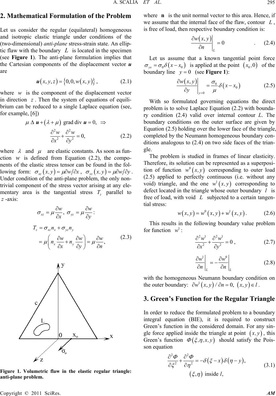

A. SCALIA ET AL. 295
2. Mathematical Formulation of the Problem
Let us consider the regular (equilateral) homogeneous
and isotropic elastic triangle under conditions of the
(two-dimensional) anti-plane stress-strain state. An ellip-
tic flaw with the boundary L is located in the specimen
(see Figure 1). The anti-plane formulation implies that
the Cartesian components of the displacement vector u
are
  
,,0,0, ,
x
yz wxyu, (2.1)
where w is the component of the displacement vector
in direction z. Then the system of equations of equili-
brium can be reduced to a single Laplace equation (see,
for example, [6])

grad div 0,   uu
22
22
0,
ww
xy


 (2.2)
where

and

are elastic constants. As soon as fun-
ction w is defined from Equation (2.2), the compo-
nents of the elastic stress tensor can be found in the fol-
lowing form:

xz
x
,yw x   ,

yz
x
,yw y   .
Under condition of the anti-plane problem, the only non-
trivial component of the stress vector arising at any ele-
mentary area is the tangential stress
z
T parallel to
z-axis:
,:
xz yz
ww
x
y
 



,
zxzxyzy
xy
Tnn
ww w
nn
x
yn




 


 

(2.3)
Figure 1. Volumetric flaw in the elastic regular triangle:
anti-plane problem.
where n is the unit normal vector to this area. Hence, if
we assume that the internal face of the flaw, contour L,
is free of load, then respective boundary condition is:


,0
L
wxy
n

 . (2.4)
Let us assume that a known tangential point force


00yx
x
x   is applied at the point


00
x
, of the
boundary line 0y

(see Figure 1):



0
0
0
,
y
wxy
x
x
y




 (2.5)
With so formulated governing equations the direct
problem is to solve Laplace Equation (2.2) with bounda-
ry condition (2.4) valid over internal contour L. The
boundary conditions on the outer surface are given by
Equation (2.5) holding over the lower face of the triangle,
completed by the Neumann homogeneous boundary con-
ditions analogous to (2.4) on two side faces of the trian-
gle.
The problem is studied in frames of linear elasticity.
Therefore, its solution can be represented as a superposi-
tion of function


0
wx,y corresponding to outer load
(2.5) applied to perfectly continuous (i.e. without any
void) triangle, and the one

1
wx,y corresponding to
defect located in the triangle whose outer boundary l is
free of load, with void L subjected to a certain tangen-
tial stress:




01
,,,wxywxyw xy. (2.6)
This results in the following boundary value problem
for function 1 w:
21 21
22
0
ww
xy


 , (2.7)
10
L
L
ww
nn



(2.8)
with the homogeneous Neumann boundary condition on
the outer boundary:


1,0,,wxy/n xyl

 .
3. Green’s Function for the Regular Triangle
In order to reduce the formulated problem to a boundary
integral equation (BIE), it is required to construct
Green’s function in the considered domain. For any sin-
gle force applied inside the triangle at point


x
,y , this
Green’s function


,,x,y  should satisfy the Pois-
son equation


22
22 ,
,inside,
x
y
l
 



 
 (3.1)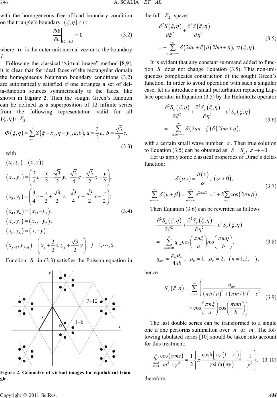

A. SCALIA ET AL. 296
with the homogeneous free-of-load boundary condition
on the triangle’s boundary

,l  :
 ,
0
l
n
 
 
 (3.2)
where n is the outer unit normal vector to the boundary
l.
Following the classical “virtual image” method [8,9],
it is clear that for ideal faces of the rectangular domain
the homogeneous Neumann boundary conditions (3.2)
are automatically satisfied if one arranges a set of del-
ta-function sources symmetrically to the faces, like
shown in Figure 2. Then the sought Green’s function
can be defined as a superposition of 12 infinite series
from the following representation valid for all

2
,E  :


12
1
33
,,,,,,,
22
jj
j
Sx yabac bc  

 

(3.3)
with





 
 

11
22
33
443 3
552 2
66
66
,,;
3333
,,;
422422
3333
,,;
42242 2
,,;
,,;
,,;
33
,,,1,,6
22
jjj j
xy xy
xy
xycy cx
xy
xycy cx
xyx y
xyx y
xyx y
x
yxcyy j.



 




 







 




(3.4)
Function S in (3.3) satisfies the Poisson equation in
Figure 2. Geometry of virtual images for equilateral trian-
gle.
the full 2 E space:




 
22
22
,,
22,,
n,m
SS
anbm .
 


 





 

(3.5)
It is evident that any constant summand added to func-
tion S does not change Equation (3.5). This non-uni-
queness complicates construction of the sought Green’s
function. In order to avoid operation with such a singular
case, let us introduce a small perturbation replacing Lap-
lace operator in Equation (3.5) by the Helmholtz operator




 
22
2
22
,,,
22,
n,m
SSS
an bm


 









 

(3.6)
with a certain small wave number

. Then true solution
to Equation (3.5) can be obtained as , 0SS


.
Let us apply some classical properties of Dirac’s delta-
function:



 
2
1
,0,
12 cos2
ni
nn n
x
x
ne n.


 



 
 

 

(3.7)
Then Equation (3.6) can be rewritten as follows





22
2
22
0
0
,,
cos cos,
;1, 2,1,2,,
4
nm
n,m
nm
nm n
SSS,
nm
qab
q n
ab


 

 
 





 
  
 



(3.8)
hence
  
22
2
,0
,
//
cos cos
nm
nm
q
S
na mb
nm
ab




 



 


 

 
 


(3.9)
The last double series can be transformed to a single
one if one performs summation over n or m. The fol-
lowing tabulated series [10] should be taken into account
for this treatment:



22 2
1
cosh 1
cos 11
,
2sinh
m
z
mz
m



















 (3.10)
therefore,

A. SCALIA ET AL. 297
 



22 222
01
cosh 1
cos cos
12sinh
m
mm
z
mz mz.
mm




 







 

 (3.11)
One thus can see from (3.9)–(3.11), with

22
bn aa

  , that
 

 

22
22 22
0
cosh
cos
,.
4sinh
n
n
nab a
na
S
na bna a




 





 





 






 (3.12)
The first term here, 0n, with asymptotically small

a represents itself a certain constant and so, according
to what was written above, can be neglected. After all
these transformations, with 0

 , the sought Green’s
function can directly be extracted from (3.12) in the fol-
lowing form:




1
cosh cos
2sinh
n
nb a
S, na.
nnba

 






 (3.13)
It is interesting to control the basic property of any
Green’s function in the two-dimensional problem: this
must possess a logarithmic singularity when

and

both tend to zero, more precisely one should control that


22
22
,14ln,
0
S~
.
 


 (3.14)
In order to prove asymptotic relation (3.14), let us take
into account the following table series [10,11]



2
1
cos 1ln 12cos,
2
0
cnc c
n
nz eeze
n
c.


 

 (3.15)
The common term in (3.13) behaves asymptotically as
n like in series (3.15) with za

 ,ca  .
Then the asymptotic behavior of expression (3.13), as


,0  , becomes:



//2/
1
22 22
2
// 22
22
cos 1ln 12cos
24
111
ln1221 coslnln,
444
naa a
n
aa
na
eee
na
ee aaa

 
 

 





 





 

 




(3.16)
that is to be proved.
At the end of this section we notice that full structure
of the sought Green’s function is given by combining
Equations (3.3) and (3.13):










12
11
cosh cos
,,, 2sinh
jj
jn
nbyanxa
xy nnba
 
 


 
 (3.17)
where the set of virtual images is given by Equation
(3.4).
4. BIE for Direct Problem
Let us come back to the elastic problem shown in Figure
1. We assume that the lower free face is loaded by a
known single force at point


0,0x, and there is an in-
ternal defect with the boundary L inside the triangle.
To resolve this problem, one can apply Green’s function
constructed in the previous section.
One can represent the unknown function


1,wxy at
arbitrary point outside the defect as an integral over its
boundary curve L, with the use of standard methods of
potential theory (see, for example, [12]):

1
11
,
L
w
wxy wdl
nn

 




 (4.1)
where both outer unit normal vector

,

 n and ele-
mentary arc of length

,dl

 are linked to point


,L 

, not to


,
x
y. It should be noted that for any
fixed point


,
x
y chosen in the elastic medium the in-
tegral in (4.1) should contain additional integration over
the outer boundary of the considered elastic domain, con-
tour l. However, the second term in such an integrand
is trivial due to boundary condition (last relation of Sec-

A. SCALIA ET AL. 298
tion 2), and the first term vanishes due to the specially
constructed Green’s function satisfying boundary condi-
tion (3.2).
Let us prove that
0
00
L
w
wdl
nn







 (4.2)
for any point

,
x
y in the elastic medium. This state-
ment can be proved directly, if one considers Green’s in-
tegral formula applied to the pair of functions:


0,w


and

,,,
x
y  inside contour L. Really, both func-
tions are regular in this domain, if point

,
x
y is out-
side L, and satisfy there the Laplace equation. Then the
application of Green’s integral formula immediately re-
sults in (4.2) [12].
Now, by summation (4.1) and (4.2), we can express


1,wxy in terms of boundary values of the full displa-
cement


,wxy and its normal derivative:


1,
,,
L
L
w
wxy wdl
nn
wdl
n

 









(4.3)
due to boundary condition (2.4).
By using the well known limiting value of the poten-
tial of double layer [12], if any

,
X
YL and contour
L is smooth, then
 



,,
,
lim,, ,,,,
2
xyXYLL
wXY
wxydlwXYdl.
nn

 





(4.4)
With such a limit
 
,,
x
yXYL, Equation (4.3) allows us to formulate the basic BIE in the form:


0
,,,,, ,,,,
2L
wXYwXYdlwXY XYL
n

 



 (4.5)
since 10 www .
For the practical usage of formulas (4.3) and (4.5), it is
helpful to write out explicitly the normal derivative of
Green’s function. If


,nn


n is the outer unit nor-
mal vector to the boundary contour L of the defect,
then






 

12 12
111
cosh sin
,
2sinh
sinhcos sgn
2sinh
jj
jj
jjn
jjj
nnbyanxa
Sx y
nnn
nanb/a
nnbyanxa y
anba



 

 
 
 





  
 
 


  

 







 

 




(4.6)
In order to complete formulation of the basic BIE (4.5)
for the direct problem, let us note that its right-hand side,
function

0,wXY can be obtained similarly to the
constructed Green’s function. Really, both Green’s func-
tion and function

0,wXY are some solutions for the
full triangle caused by a point Dirac’s outer applied force.
The only difference is that for

0,wXY Dirac’s delta
is applied over the boundary contour, not inside the do-
main. Therefore, function

0,wXY can directly be
obtained from representation (3.17) for Green’s function,
if one sets there point

,
x
y approaching the boundary
point


0,0x, and replaces

,

 by

,
X
Y. Besides,
in Equation (3.1) there is sign “minus” in front of Dirac’s
delta in the right-hand side, hence function


0,wXY
has to be taken with opposite sign. It should also be
noted that with the real source image in Figure 2 tending
to the boundary point


0,0x, where the outer force is
applied, in fact a pair of virtual images (one real and one
imaginary) approaches the same point

0,0x. For this
reason the final resulting limit value should be taken in
half. By arranging such a limit, one can obtain the fol-
lowing representation for

0,wXY:





6
00
11
cosh /
,cos
4sinh/
k
k
kn
nb Yya
wXYnXx a
nnba


 









 




 (4.7)

A. SCALIA ET AL. 299
for any

,
X
Y inside the triangle. Note that the dimen-
sion of the set of virtual images here is in two times less
when compared to that in Equation (3.17):





11 0
0
22 0
0
33 0
33
,,0;
333
,,;
4242
333
,, ;
4242
33
,;
22
33
,,,1,,3
22
kkk k
xy x
x
xyc cx
x
xyc cx
ac bc
x
yxcyc k.



 










 




(4.8)
5. Reconstruction Problem and Some
Numerical Results
If function

0,wxy,


,
x
yL is determined from
BIE (4.5), the displacement field at arbitrary point of the
elastic medium can be calculated by using Equation
(4.3):
  
0
,,,
L
wxyw xywdl
n



 
 (5.1)
where the quantity n


 is given by Equation (4.6).
After that, the components of the stress tensor can be cal-
culated as xz wx



, yz wy

 . One thus can
calculate all physical quantities at arbitrary point


,
x
y
inside the medium. In particular, the shape of the lower
boundary surface


,0wx l

is directly extracted from
Equation (5.1). From that representation, we can easily
observe the contribution given by the two physically dif-
ferent components:
1) the deformation of the boundary in the perfect (i.e.
free of any void) triangle under the applied force 0

,
that is given by the first term in (5.1);
2) the contribution given by the influence of presence
of the flaw, the second integral term in (5.1).
The latter can be calculated as:
 

12
00
11
1
,0 ,coshsin
2sinh
sinhcossgn ,
j
j
jn
L
jj
j
by
x
Fx Fxwnnn
anbaa a
by x
nnnydl
aa



 






 


 





 
 


 





(5.2)
and gives, as has been said above, the contribution to the
deformation of the lower boundary surface given by the
defect itself.
The inverse reconstruction problem is formulated as
follows. Let us assume that a defect of unknown position
and shape is located somewhere inside the elastic trian-
gle. Let us apply a concentrated single force 0

at a
certain point on the lower face 0y and measure the
deformation of this lower face. Then, by knowing this
measured deformation, it is necessary to predict the posi-
tion, size, and form of the defect. It is obvious that ma-
thematically the problem is to determine contour L
from the known function

0
F
x. Since another un-
known function


X,YL
wX,Y

is involved in all mathe-
matical formulas, this means that mathematically one
needs to solve the system of two integral Equations (4.5)
and (5.2). This system is nonlinear with respect to any
defining equation describing contour L. Moreover, since
Equation (5.2) is of the first kind, the considered system
is ill-posed (see [13]).
The proposed approach is founded on the collocation
technique (see, for example, [12]). If contour L is known,
then one can arrange a dense set of nodes


,,
mm

1, ,mN

belonging to this contour:

,,
mm Lm


,
which subdivides it to N small intervals of length m
l.
Then the approximate numerical solution to Equation
(4.5) can be obtained by solving the linear algebraic sys-
tem:

 



0
1
6
00
0
11
,1,,,,, ,,,,
1coshcos ,
4sinh
N
im mimmmmxmmmymm
m
ikk
kn
aww iN wwnn nn
wnbyanxxa
nnba

 

 



 

  





(5.3a)
with the elements of matrix

im
a being given as follows:

A. SCALIA ET AL. 300


12
11
1;if :
2
cosh sin
2sinh
sinhcossgn .
ii
mj mj
m
im m
jn
mj mj
mmj
aim
by
x
l
annn
anbaaa
by x
nn ny
aa











 


 





 
 


 



 (5.3b)
This system is constructed so that the set of the “inner”
discrete integration points




,
mm
 , over which the
integration is being performed, coincides with the set of
the "outer" nodes



,
ii
xy

, which are used to
provide the equality between the left- and the right-hand
sides in (5.3). This implies that the full set of 12 virtual
images is given by expression (3.4) where one should set
,
ii
xy

.
It should also be noted that elements im a of a long
structure are excluded from the diagonal elements (the
case im). These elements correspond to the case
when
 
,,
X
Y   in the kernel of integral (4.5). It
can easily be proved that these elements remain always
bounded for any smooth line L, being related to the
curvature of the contour at point

,
X
Y. However, the
contribution of such elements to the full sum (5.3) is
small (as

0
m
max l) when compared with the con-
tribution of the “outer” term in (5.3) outside the integral,
which in the discrete form results in the diagonal element
12
ii
a

. Such a treatment allows us to write out the sys-
tem (5.3) in a shorter form.
When solving the posed reconstruction problem, in
practice, the measurements on the deformation of the
lower boundary surface cannot be carried out with abso-
lute precision. This predetermines the input data to be
known with a certain error. Therefore, the proposed al-
gorithm should provide stability with respect to small
perturbations of the input data.
All above developed formulas are valid for arbitrary
smooth contour L. However, if the flaw is an elliptic
cylinder with the semi-axes
A
and B, with its center
being located at the point

,ch and with the angle of
inclination

respectively axis
x
, then the above for-
mulas can be written in a more concrete form since


 

 

222 2
222 2
cos ,
sin cos
sin ;
sin cos
2
05;
m
m
mm
m
m
mm
m
AB
d
AB
AB
h
AB
i, .
N













 

 



 


 


(5.4)
Under such conditions the reconstruction problem be-
comes five-dimensional, because this is to seek five pa-
rameters ,,, ,d h A B

.
Our approach is founded on an explicit (numerical)
resolution of system (5.3) considered as a linear alge-
braic system for quantities m w. Let us represent this
system in the operator form








000
,, ,,,1,,,
imm i
wwaw w wwimN A A
(5.5)
then its inversion is

10 10
, .
ii
www w

AA (5.6)
Obviously, operator 1

A depends on five parameters:


11
,, , ,dhAB


AA, hence the substitution of (5.6)
into (5.2) results, in the discrete form, in the overdeter-
mined system of nonlinear equations for parameters
,,,,d h A B

:





12
111
10*
0
*
1cosh sin
2sinh
sinhcossgn, ,,,,
1,,, 0,,
Nmj mj
m
mjn
mj mj
mmjmq
m
q
by x
nn n
anbaa a
by x
nnnydhABwlFx
aa
qQxa






 




 


 





 
 
 

 






A

(5.7)

A. SCALIA ET AL. 301
where Q control points


,0 ,0,
**
qq
x
xa all belong
to the lower face of the triangle. It should be noted that in
the case when observation point

,
x
y moves to any
point

,0
*
q
x belonging to the lower boundary of the
triangular domain the number of virtual images


,
j
j
x
y
given by Equation (3.4) reduces again in two times.
Equation (5.7) can be resolved by a minimization of
the discrepancy functional [14]:





12
1111
10
*
0
min,,,,, ,,,,
cosh
sin sinh
cos sgn
,, , ,
.
2sinh /
QNmj
m
qmjn
mj
mj
m
mj
mj
m
m
q
dhABdhAB
by
nn
a
by
x
nnn
aa
x
ny
a
dhABwl
Fx
anba















 


















 

 





A
(5.8)
It is obvious that in the case of exact input data zero
minimal value of  corresponds to exact solution of
the inverse reconstruction problem. However, the prob-
lem under consideration is nonlinear, hence nobody can
guarantee uniqueness of the solution. It should also be
noted that, in order to simulate a small error in the input
data, we first solve respective direct problem when the
shape of the defect is known, and then perturb the ob-
tained solution by a random perturbation. So constructed
function 0
F
is used as the approximate input data.
For the minimization of functional  we used in our
numerical experiments a version of the random search
method [15].
Some examples of the reconstruction are demonstrated
in Tables below. For all examples we used 1,c

50N, 100Q, 00x.
Here in Table 1 two different flaws located at the
same position are considered—a circle and an ellipse
directed horizontally, both reconstructions—with exact
input data. It is interesting to note that the slope angle for
the circle is of no importance in the reconstruction pro-
cess, and the reconstructed value of

plays no role.
Then we studied the stability of the proposed algori-
thm if the input data is given with an error. As commen-
ted above, we add some small perturbation to the solu-
tion of respective direct problem. More precisely, each
value of the lower face deformation 0
F
is recalculated
to a new value by the following formula:

00
121
F
F    

,
where

is the magnitude of the error (which being
Table 1. Results of the reconstruction with e xac t input data.
Input data
error d h A B θ Type of result
0% 0.000
-0.007
0.300
0.296
0.150
0.148
0.150
0.152
0.000
0.617
Exact
restored
0% 0.000
0.009
0.300
0.308
0.250
0.253
0.150
0.157
0.000
-0.002
Exact
restored
multiplied by 100 can also be expressed in percents), and

is a random number distributed uniformly over inter-
val

 1,0 . Some results of such a numerical simulation
are shown in Table 2.
It is interesting to notice here that the second example
is related to the case when the elliptic flaw is located ver-
tically: in fact, the reconstructed flaw possesses the same
property, despite inversion of its principal axes.
Further increase in the error of the input data results in
the following table:
Here we notice once again that for the first defect in
Table 3 the last reconstructed parameter

plays no
role, as the flaw is in fact a circle. One thus can admit
that this flaw is restored quite well, despite the error in
the input data.
From the presented results of the numerical simulation,
as well as from many other reconstruction examples per-
formed, we can come to some important conclusions:
1) Generally, precision of the reconstruction is less de-
pendent on the error of the input data than on geometry
of the void.
2) The precision of the reconstruction as a rule is good.
In some cases almost the same results are obtained with
formally different reconstructed geometries. However,
with a certain precision, the reconstructed object gives
the same original geometry but with another combination
of the reconstructed parameters.
3) The worst precision takes place in the reconstruc-
tion of prolate ellipses, i.e. with low aspect ratio BA
(see the second example in Table 3 and the second one
in Table 2). One can state the following rule natural
Table 2. Results of the reconstruction with relative error
5% in the input data.
Input
data errord h A B θ Type of result
5% 0.200
0.205
0.150
0.144
0.100
0.102
0.030
0.036
π/4=0.785
0.797
Exact
restored
5% 0.200
0.196
0.150
0.154
0.200
0.109
0.100
0.208
π/2=1.571
0.069
Exact
restored
Table 3. Results of the reconstruction with relative error
10% in the input data.
Input
data errord h A B θ Type of result
10% 0.250
0.265
0.250
0.270
0.100
0.095
0.100
0.113
0
0.514
Exact
restored
10% 0.150
0.131
0.300
0.227
0.200
0.176
0.050
0.068
- π/4
-0.882
Exact
restored

A. SCALIA ET AL. 302
from physical point of view: the more prolate is the void
the less is the precision of the reconstruction.
6. Acknowledgements
The paper has been supported in part by Italian Ministry
of University (M.U.R.S.T.) through its national and local
(60%) projects. The work is also supported by Russian
Foundation for Basic Research (RFBR), Project 10-01-
00557.
7. References
[1] A. Friedman and M. Vogelius, “Determining Cracks by
Boundary Measurements,” Indiana University Mathe-
matics Journal, Vol. 38, No. 3, 1989, pp. 527-556.
doi:10.1512/iumj.1989.38.38025
[2] G. Alessandrini, E. Beretta and S. Vessella, “Determining
Linear Cracks by Boundary Measurements: Lipschitz
Stability,” SIAM Journal on Mathematical Analysis, Vol.
27, No. 2, 1996, pp. 361-375.
doi:10.1137/S0036141094265791
[3] A. B. Abda et al., “Line Segment Crack Recovery from
Incomplete Boundary Data,” Inverse Problems, Vol. 18,
No. 4, 2002, pp. 1057-1077.
doi:10.1088/0266-5611/18/4/308
[4] S. Andrieux and A. B. Abda, “Identification of Planar
Cracks by Complete Overdetermined Data: Inversion
Formulae,” Inverse Problems, Vol. 12, No. 5, 1996, pp.
553-563. doi:10.1088/0266-5611/12/5/002
[5] T. Bannour, A. B. Abda and M. Jaoua, “A Semi-Explicit
Algorithm for the Reconstruction of 3D Planar Cracks,”
Inverse Problems, Vol. 13, No. 4, 1997, pp. 899-917.
doi:10.1088/0266-5611/13/4/002
[6] A. S. Saada, “Elasticity: Theory and Applications,” 2nd
Edition, Krieger, Malabar, Florida, 1993.
[7] N. I. Muskhelishvili, “Some Basic Problems of the Ma-
thematical Theory of Elasticity,” Kluwer, Dordrecht,
1975.
[8] R. Courant and D. Hilbert, “Methods of Mathematical
Physics,” Interscience Publishing, New York, Vol. 1,
1953.
[9] L. Cremer and H. A. Müller, “Principles and Applications
of Room Acoustics,” Applied Science, London, Vol. 1, 2,
1982.
[10] I. S. Gradshteyn and I. M. Ryzhik, “Table of Integrals,
Series, and Products,” 5th Edition, Academic Press, New
York, 1994.
[11] H. Hardy, “Divergent Series,” Oxford University Press,
London, 1956.
[12] M. Bonnet, “Boundary Integral Equations Methods for
Solids and Fluids,” John Wiley, New York, 1999.
[13] A. N. Tikhonov and V. Y. Arsenin, “Solutions of Ill-
Posed Problems,” Winston, Washington, 1977.
[14] P. E. Gill, W. Murray and M. H. Wright, “Practical Op-
timization,” Academic Press, London, 1981.
[15] M. Corana et al., “Minimizing Multimodal Functions of
Continuous Variables with the Simulated Annealing Al-
gorithm,” ACM Transactions on Mathematical Software,
Vol. 13, No. 3, 1987, pp. 262-280.
doi:10.1145/29380.29864