J. Biomedical Science and Engineering, 2009, 2, 184-189
Published Online June 2009 in SciRes. http://www.scirp.org/journal/jbise
JBiSE
Identifying species-specific subsequences in
bacteria transcription terminators-A
machine learning approach
Bao-Hua Gu1, Yi Sun1
1School of Computing Science, Simon Fraser University, 8888 University Drive, Burnaby, BC, Canada.
Received 24 March 2008; revised 10 March 2009; accepted 5 April 2009.
ABSTRACT
Transcription Terminators (TTs) play an impor-
tant role in bacterial RNA transcription. Some
bacteria are known to have Species-Specific
Subsequences (SSS) in their TTs, which are be-
lieved containing useful clues to bacterial evolu-
tion. The SSS can be identified using biological
methods which, however, tend to be costly and
time-consuming due to the vast number of sub-
sequences to experiment on. In this paper, we
study the problem from a computational per-
spective and propose a computing method to
identify the SSS. Given DNA sequences of a tar-
get species, some of which a re known to contain
a TT while others not, our method uses machine
learning techniques and is done in three steps.
First, we find a ll frequent subseq uences from th e
given sequences, and show that this can be effi-
ciently done using generalized suffix trees. Sec-
ond, we use these subsequences as features to
characterize the original DNA sequences and
train a classification model us ing Support Vector
Machines (SVM) , one of the currently most effec-
tive machine learning techniques. Using the pa-
rameters of the re sult ing SVM model, w e define a
measure called subsequence specificity to rank
the frequent subsequences, and output the one
with the highest rank as the SSS. Our experi-
ments show that the SSS found by the proposed
method are very close to those determined by
biological experiments. This suggests that our
method, though purely computational, can help
efficiently locate the SSS by effectiv ely narro wing
down the search space.
1. INTRODUCTION
Bacterial genomes are organized into units of expression
that are bounded by sites where transcription of DNA
into RNA is initiated and terminated. The former site is
called Transcription Promoter, which determine what
region and which strand of DNA will be transcribed into
RNA. The later site is called Transcription Terminator
(TT), which is a stop signal to terminate the transcription
process [1].
Although the mechanism of transcription termination
in bacteria is rho-independent, or intrinsic, the TTs in
different bacteria have a common hairpin-like RNA
structure as shown in Figure 1: typically a stem-loop
structure with dyadic stempairing high in guanine (G)
and cytosine (C) residue content, followed by a uracil-
rich (U) stretch of sequence proximal to the termination
site [2].
This particular RNA structure is encoded in the certain
region of the corresponding DNA sequence. It is well
known that the DNA sequences of some bacteria have
species-specific subsequences (SSS) for the TTs. That is,
the subsequence appears significantly more frequently in
certain species than in others. For example, for bacte-
rium Neisseria Meningitidis, the SSS is GCCGTCTGAA,
while for bacterium Haemophilus Influenzae, the SSS is
AAGTGCGGT [3]. Having found many DNA sequences
of TTs of many bacteria, biologists are wondering
whether these bacteria also have such SSS. The biologi-
cal motivation behind is that the SSS might provide bet-
ter understanding of the terminator evolution and how it
functions in genetic exchange between pathogens.
Of course, the SSS can be determined by biological
experiments. However, such experiments tend to be
costly and time-consuming because every subsequence
has to be examined and the number of such subse-
quences can be prohibitively large due to the length of
the DNA sequences. To overcome the difficulty, biolo-
gists typically apply domain knowledge to narrow down
the search space. However, the process of obtaining such
knowledge itself would also be time-consuming and
highly expensive if they are not available yet. Therefore,
it is desirable to study alternative ways to effectively
identify the SSS from the given DNA TT sequences.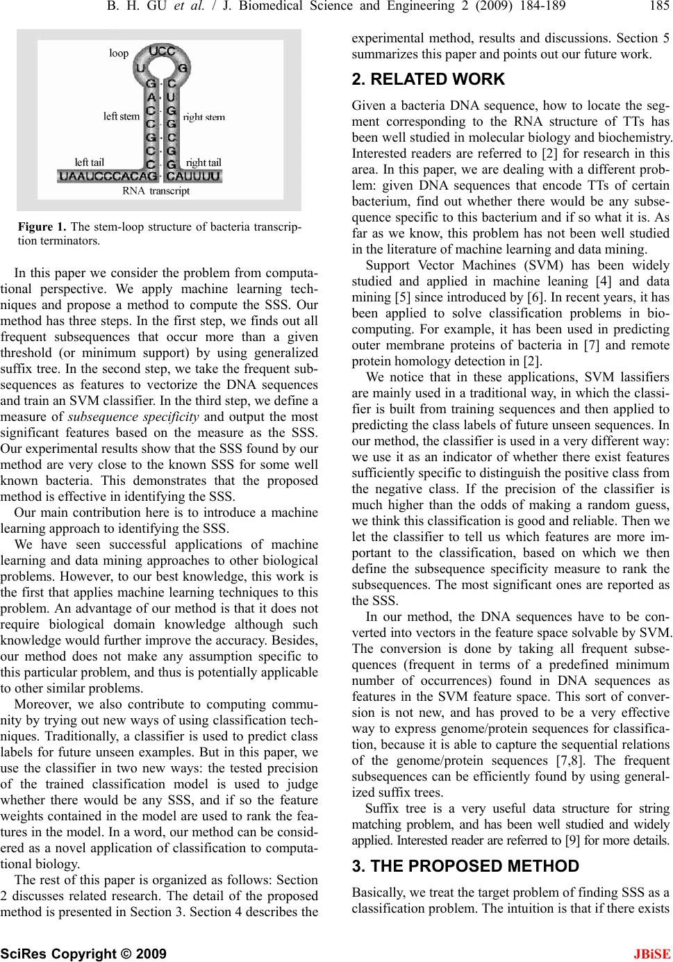

B. H. GU et al. / J. Biomedical Science and Engineering 2 (2009) 184-189 185
SciRes Copyright © 2009 JBiSE
Figure 1. The stem-loop structure of bacteria transcrip-
tion terminators.
In this paper we consider the problem from computa-
tional perspective. We apply machine learning tech-
niques and propose a method to compute the SSS. Our
method has three steps. In the first step, we finds out all
frequent subsequences that occur more than a given
threshold (or minimum support) by using generalized
suffix tree. In the second step, we take the frequent sub-
sequences as features to vectorize the DNA sequences
and train an SVM classifier. In the third step, we define a
measure of subsequence specificity and output the most
significant features based on the measure as the SSS.
Our experimental results show that the SSS found by our
method are very close to the known SSS for some well
known bacteria. This demonstrates that the proposed
method is effective in identifying the SSS.
Our main contribution here is to introduce a machine
learning approach to identifying the SSS.
We have seen successful applications of machine
learning and data mining approaches to other biological
problems. However, to our best knowledge, this work is
the first that applies machine learning techniques to this
problem. An advantage of our method is that it does not
require biological domain knowledge although such
knowledge would further improve the accuracy. Besides,
our method does not make any assumption specific to
this particular problem, and thus is potentially applicable
to other similar problems.
Moreover, we also contribute to computing commu-
nity by trying out new ways of using classification tech-
niques. Traditionally, a classifier is used to predict class
labels for future unseen examples. But in this paper, we
use the classifier in two new ways: the tested precision
of the trained classification model is used to judge
whether there would be any SSS, and if so the feature
weights contained in the model are used to rank the fea-
tures in the model. In a word, our method can be consid-
ered as a novel application of classification to computa-
tional biology.
The rest of this paper is organized as follows: Section
2 discusses related research. The detail of the proposed
method is presented in Section 3. Section 4 describes the
experimental method, results and discussions. Section 5
summarizes this paper and points out our future work.
2. RELATED WORK
Given a bacteria DNA sequence, how to locate the seg-
ment corresponding to the RNA structure of TTs has
been well studied in molecular biology and biochemistry.
Interested readers are referred to [2] for research in this
area. In this paper, we are dealing with a different prob-
lem: given DNA sequences that encode TTs of certain
bacterium, find out whether there would be any subse-
quence specific to this bacterium and if so what it is. As
far as we know, this problem has not been well studied
in the literature of machine learning and data mining.
Support Vector Machines (SVM) has been widely
studied and applied in machine leaning [4] and data
mining [5] since introduced by [6]. In recent years, it has
been applied to solve classification problems in bio-
computing. For example, it has been used in predicting
outer membrane proteins of bacteria in [7] and remote
protein homology detection in [2].
We notice that in these applications, SVM lassifiers
are mainly used in a traditional way, in which the classi-
fier is built from training sequences and then applied to
predicting the class labels of future unseen sequences. In
our method, the classifier is used in a very different way:
we use it as an indicator of whether there exist features
sufficiently specific to distinguish the positive class from
the negative class. If the precision of the classifier is
much higher than the odds of making a random guess,
we think this classification is good and reliable. Then we
let the classifier to tell us which features are more im-
portant to the classification, based on which we then
define the subsequence specificity measure to rank the
subsequences. The most significant ones are reported as
the SSS.
In our method, the DNA sequences have to be con-
verted into vectors in the feature space solvable by SVM.
The conversion is done by taking all frequent subse-
quences (frequent in terms of a predefined minimum
number of occurrences) found in DNA sequences as
features in the SVM feature space. This sort of conver-
sion is not new, and has proved to be a very effective
way to express genome/protein sequences for classifica-
tion, because it is able to capture the sequential relations
of the genome/protein sequences [7,8]. The frequent
subsequences can be efficiently found by using general-
ized suffix trees.
Suffix tree is a very useful data structure for string
matching problem, and has been well studied and widely
applied. Interested reader are referred to [9] for more details.
3. THE PROPOSED METHOD
Basically, we treat the target problem of finding SSS as a
classification problem. The intuition is that if there exists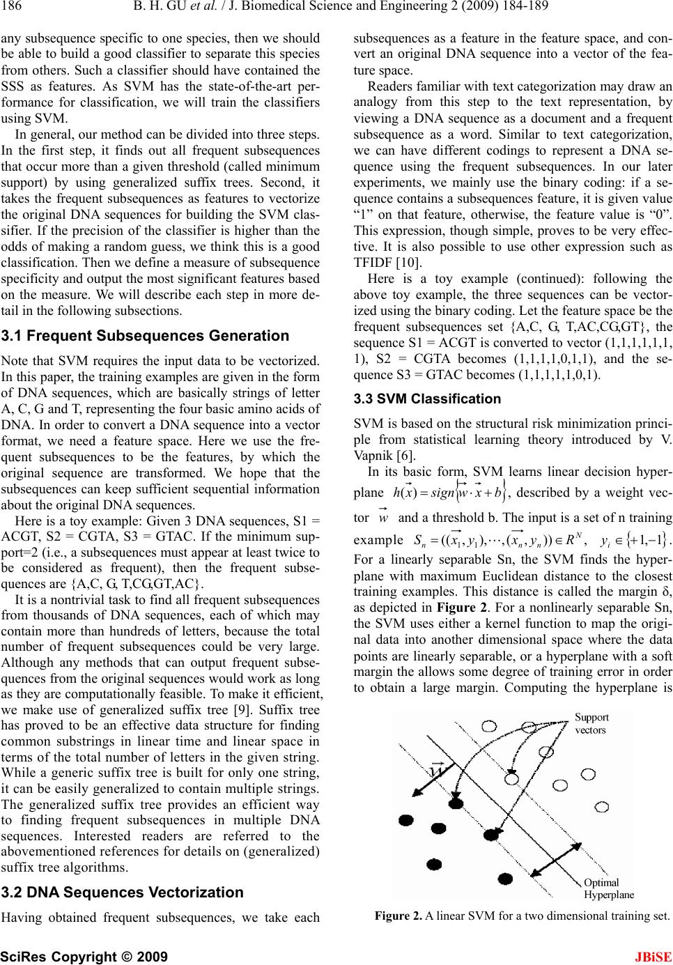

186 B. H. GU et al. / J. Biomedical Science and Engineering 2 (2009) 184-189
SciRes Copyright © 2009 JBiSE
any subsequence specific to one species, then we should
be able to build a good classifier to separate this species
from others. Such a classifier should have contained the
SSS as features. As SVM has the state-of-the-art per-
formance for classification, we will train the classifiers
using SVM.
In general, our method can be divided into three steps.
In the first step, it finds out all frequent subsequences
that occur more than a given threshold (called minimum
support) by using generalized suffix trees. Second, it
takes the frequent subsequences as features to vectorize
the original DNA sequences for building the SVM clas-
sifier. If the precision of the classifier is higher than the
odds of making a random guess, we think this is a good
classification. Then we define a measure of subsequence
specificity and output the most significant features based
on the measure. We will describe each step in more de-
tail in the following subsections.
3.1 Frequent Subsequences Generation
Note that SVM requires the input data to be vectorized.
In this paper, the training examples are given in the form
of DNA sequences, which are basically strings of letter
A, C, G and T, representing the four basic amino acids of
DNA. In order to convert a DNA sequence into a vector
format, we need a feature space. Here we use the fre-
quent subsequences to be the features, by which the
original sequence are transformed. We hope that the
subsequences can keep sufficient sequential information
about the original DNA sequences.
Here is a toy example: Given 3 DNA sequences, S1 =
ACGT, S2 = CGTA, S3 = GTAC. If the minimum sup-
port=2 (i.e., a subsequences must appear at least twice to
be considered as frequent), then the frequent subse-
quences are {A,C, G, T,CG,GT,AC}.
It is a nontrivial task to find all frequent subsequences
from thousands of DNA sequences, each of which may
contain more than hundreds of letters, because the total
number of frequent subsequences could be very large.
Although any methods that can output frequent subse-
quences from the original sequences would work as long
as they are computationally feasible. To make it efficient,
we make use of generalized suffix tree [9]. Suffix tree
has proved to be an effective data structure for finding
common substrings in linear time and linear space in
terms of the total number of letters in the given string.
While a generic suffix tree is built for only one string,
it can be easily generalized to contain multiple strings.
The generalized suffix tree provides an efficient way
to finding frequent subsequences in multiple DNA
sequences. Interested readers are referred to the
abovementioned references for details on (generalized)
suffix tree algorithms.
3.2 DNA Sequences Vectorization
Having obtained frequent subsequences, we take each
subsequences as a feature in the feature space, and con-
vert an original DNA sequence into a vector of the fea-
ture space.
Readers familiar with text categorization may draw an
analogy from this step to the text representation, by
viewing a DNA sequence as a document and a frequent
subsequence as a word. Similar to text categorization,
we can have different codings to represent a DNA se-
quence using the frequent subsequences. In our later
experiments, we mainly use the binary coding: if a se-
quence contains a subsequences feature, it is given value
“1” on that feature, otherwise, the feature value is “0”.
This expression, though simple, proves to be very effec-
tive. It is also possible to use other expression such as
TFIDF [10].
Here is a toy example (continued): following the
above toy example, the three sequences can be vector-
ized using the binary coding. Let the feature space be the
frequent subsequences set {A,C, G, T,AC,CG,GT}, the
sequence S1 = ACGT is converted to vector (1,1,1,1,1,1,
1), S2 = CGTA becomes (1,1,1,1,0,1,1), and the se-
quence S3 = GTAC becomes (1,1,1,1,1,0,1).
3.3 SVM Classification
SVM is based on the structural risk minimization princi-
ple from statistical learning theory introduced by V.
Vapnik [6].
In its basic form, SVM learns linear decision hyper-
plane


bxwsignxh )( , described by a weight vec-
tor w and a threshold b. The input is a set of n training
example ,)),(,),,(( 11
N
nnn RyxyxS  

 1,1



i
y.
For a linearly separable Sn, the SVM finds the hyper-
plane with maximum Euclidean distance to the closest
training examples. This distance is called the margin δ,
as depicted in Figure 2. For a nonlinearly separable Sn,
the SVM uses either a kernel function to map the origi-
nal data into another dimensional space where the data
points are linearly separable, or a hyperplane with a soft
margin the allows some degree of training error in order
to obtain a large margin. Computing the hyperplane is
Figure 2. A linear SVM for a two dimensional training set.

B. H. GU et al. / J. Biomedical Science and Engineering 2 (2009) 184-189 187
SciRes Copyright © 2009 JBiSE
equivalent to solving an optimization problem. The re-
sulting model is actually the decision hyperplane, ex-
pressed by w and b.
Note that the resulting weights can be actually viewed
as a ranking of the features: a positive (negative) weight
means the corresponding feature values contribute to the
positive (negative) class; the larger the absolute weight
value, the more important the feature is to the classifica-
tion; weights of zero or very small values have little
contribution to classification. Later we will use this
ranking information to define what we call the measure
of subsequence specificity.
We decide to use SVM for classification because it
has proved to have a number of advantages over other
classification algorithms. First, it can easily handle very
high dimensional input space [11]. Second, it works well
when the problem contain few irrelevant features [11].
Third, it does not require feature selection as a preproc-
essing step, because it can automatically ignore irrele-
vant features during the optimization [11]. Fourth, the
weights contained in the resulting SVM model can be
used to rank the features. All these are essential to solv-
ing the target problem.
In this paper, we use the popular SVM-light imple-
mentation of SVM [12]. Note that when training SVM
classifier, one can select a kernel function suitable for
the studied problem. Motivated by the fact that text
documents are in general linearly separable [11], in our
later experiments we only consider linear SVM model
which is used by default in SVMlight.
3.4 Measure of Good Classifiers
Usually the performance of a classifier is measured by
classification accuracy, precision and/or recall. They are
defined based on a confusion matrix as shown in Table I.
The Precision of the positive class is defined as P=
TP=(TP+FP), while the Recall of the positive class is
defined as R=TP/(TP+FN). The overall Accuracy is de-
fines as A=(TP+TN)/(TP+FP+TN+FN). In our method,
the performance of SVM classifier is not measured by
the overall accuracy, because negative training se-
quences would be much more than those positives, and
the overall accuracy would be heavily affected by the
overwhelming negatives.
Besides, as our goal is to identify the specific subse-
quences in positive species, we hope to maximize the
precision (i.e., the probability of the classifier making a
correct prediction is high). Therefore, we will only use
precision as the measure of classifier’s performance. At
the same time, we will report corresponding recalls for
reference. Note that the precision of the classifier should
be higher than the odds that one makes a random guess
for the positive class label, in order to be considered as a
good classification. Otherwise, the classifier does not
make sense. For example, if a training data set contains
Table 1. Confusion matrix in classification.
Actual number of
positive examples
Actual number of
negative examples
Number of examples
classified as positiveTrue Positive (TP) False Positive (FP)
Number of examples
classified as negativeFalse Negative (FN) True Negative (TN)
100 positive examples and 100 negative examples, if one
randomly guesses for the class label of any of the 200
examples, the probability of making a correct guess is
obviously 50%. If a classifier than a random guess, then
the classifier is useless. A bad classification may suggest
that the information contains in the training examples is
probably insufficient for the classifier to distinguish the
positive examples from the negative examples.
In our method, we take this as an indication that the
positive species probably contains no SSS. In other
words, we consider a classifier is good only when its
precision is much higher than the random guess odds. In
our later experiments, the precision is obtained by test-
ing against a reserved portion of the total data, which is
unseen during the classifier is trained.
3.5 Subsequence Specificity Measure
Note that the resulting classifier will not be used as usual
to predict class label for an unseen sequence. Remember
the task here is to identify the SSS. For this purpose, we
make use of the weights of features in the SVM model,
to define what we call subsequence specificity to meas-
ure how specific a subsequence f is to the positive spe-
cies as follows:
spec(f)=svm_weight(f)×support(f,+)
×confidence(f,+).
here weight (f) is the weight of feature f obtainable from
the learned SVM model, support (f,+) is a measure of
how many sequences of positive species contain f, and
confidence(f,+) is a measure of how many sequences
that contain f belong to positive species.
The definition of the subsequence specificity is based
on the following observations and expectations:
1) An SSS should occur frequently in the positive
species. This means it should have a high support.
2) An SSS should occur more frequently in the posi-
tive species than in the negative species. This means it
should have a high confidence.
3) Having a high support and/or a high confidence
does not necessarily mean a high distinguishing power,
while this can be reliably judged by the feature weights
in SVM model.
4) SVM may give more weight on features having low
support and/or confidence. This means the weights alone
are insufficient to measure the specificity.
5) Each of the three quantities alone characterizes the
subsequence specificity from an unique angle. Combing

188 B. H. GU et al. / J. Biomedical Science and Engineering 2 (2009) 184-189
SciRes Copyright © 2009 JBiSE
them together should be able to give a more accurate
characterization of the specificity, and thus is expected
to be a more reliable measure.
4. EVALUATION
4.1 The Data Set
The data set used in this project is provided by the Brink-
man Libratory of SFU Molecular Biology and Biochemis-
try Department. It contains known rho-independent tran-
scription terminator sequences for 42 bacteria genomes.
The source of the data set is The Institute for Genomic
Research (TIGR). Each record of the data set contains one
terminator sequence (including left tail, stem and loop, and
right tail) and the taxonomy id of the corresponding bacte-
rium. The total number sequences is 12763, and 18 species
have less than 100 terminator sequences.
Besides, we are also provided with a file containing
the taxonomy information of all bacteria species. Figure
3 shows the taxonomy tree for the 42 bacteria, obtained
from the file. The tree shows the evolution paths for the
42 bacteria. Each node in the tree represents a bacterium
species, and marked by its taxonomy id. The leaf nodes
are enclosed by a parenthesis. Note that among the 42
bacteria, 41 are at leaf nodes, except species 562, which
has species 83334 as its children. This is the only pair of
species that has a direct parent-children relationship in
the given data set.
The task is to identify those DNA subsequences that
are specific to certain species. The hope is that this
should provide a better understanding of bacteria evolu-
tion and how it plays a role in genetic exchange be-
tween pathogens. Note that for a given species, it does
not necessarily have any subsequences specific to it.
Also, when talking about the specificity, one should
consider the corresponding scope. That is, with respect
to which species a subsequence is considered specific.
For example, a subsequence can be specific to bacte-
rium A with respect to another bacterium B. Also, the
subsequence can be specific to bacterium A with respect
to all other bacteria.
Among the 42 species, we evaluate our methods on
four bacteria whose SSS for the TTs are already known
biologically. The four species are: Haemophilus influ-
enzae, Neisseria meningitidis, Pasteurella multocida,
and Pseudomonas aeruginosa [3]. As the SSS for the
four bacteria are all found in the left inverted repeat (i.e.,
the left stem) of corresponding TTs, we will also use the
left stem of each TT sequence to find the SSS. For each
of the four species, we employ the one-against-
all-others approach to build classifier by taking all its
TT sequences (the left stems) as positive sequences
while those of the other 41 species as negative se-
uences. q
4.2. Experimental Methodology
All experiments are done using 5-fold cross validation.
Averaged values over the five round experiments are
reported. The linear classifiers are trained using SVM-
light default settings. The frequent subsequences are
obtained from the positive training sequences by setting
the minimum support to be 1% of the total number of
positive sequences (and the absolute support number no
less than 2). These frequent subsequences represent sta-
tistically significant features with regard to the positive
species, while resulting in substantially lower dimen-
sions compared to the feature space of all potential sub-
sequences. The classification performance is evaluated
by the precisions, while the corresponding recalls are
reported for reference.
4.3 Experimental Results
The results are given in Table II, from which we can see
that the precisions for all the four species are signifi-
cantly higher than the respective random guess odds.
This implies that there are subsequence features that can
distinguish the positive species from all the others. We
then output the top 10 subsequences based on the sub-
sequence specificity measure. The results are given in
Ta b l e 2. In Ta ble 3, the resulting subsequences that are
the closest to the known SSS are underlined.
We can see that for species Pasteurella multocida and
Pseudomonas aeruginosa, the underlined subsequences
are exactly the same as the known SSS. For the Haemo-
philus influenzae and Neisseria memingitidis, our results
are very close to the known SSS: the underlined ones are
very close to the known SSS. In all cases, our top 10
subsequences are almost the substrings of the known
SSS. This shows that our method is rather effective in
finding SSSs. Note that the known SSS are found by
applying biological domain knowledge [3], for example,
discarding those biologically meaningless subsequences
and/or limiting the length of the subsequences, which is
not considered in our method. Therefore, it can be ex-
pected that our method can be improved by incorporat-
ing domain knowledge.
Table 2. Classification performance for the four bacteria.
Name of the
Positive
Species
# of Freq
Subseq
Classifier
Precision
Classifier
Recall
Odds of
Random
Guess
Haemophilus
influenzae 325 55.81% 14.18% 3.19%
Neisseria
meningitidis 360 99.61% 50.67% 3.62%
Pasteurella
multocida 389 48.0% 1.09% 3.73%
Pseudomonas
aeruginosa 296 67.77% 9.34% 4.28%

B. H. GU et al. / J. Biomedical Science and Engineering 2 (2009) 184-189 189
SciRes Copyright © 2009 JBiSE
Table 3. The top 10 subsequences with the greatest specificity values for the four species.
The Subsequences found for each Bacterium
Top spec
rank Haemophilus Influenzae Neisseria meningitidis Pasteurella multocida Pseudomonas aeruginosa
1 TGCGGT GCCGTC TGCGGTC GCCCCGC
2 GTGCGGT CGTCTG GTGCGGTC CCCCGC
3 GTGCGG CGTCTGA ACCGCAC GCCCCG
4 CGCACTT CGTCTGAA CCGCAC CCCGC
5 CCGCACT GCCGTCT TGCGGT GCCCC
6 CCGCACTT CCGTCTG GTGCGGT CCCGGC
7 GCGGT CCGTCTGA GCGGTC GCCC
8 CGCACT CGTCT GGCGAA GCC
9 TGCGG CCGTCTGAA ACCGCA GGCGACC
1 0 TGCGGTT GTCTGA CGGTC GGC
actual SSS AAGTGCGGT GCCGTCTGAA GTGCGGT GCCCCGC
5. CONCLUSION
In this paper, our goal is to find the species-specific
subsequences for bacteria transcription terminators. By
treating the problem as a classification problem, we
propose a solution based on frequent subsequences and
Support Vector Machines. We first find frequent subse-
quences from the terminator DNA sequences of the posi-
tive species. We then take all such subsequences as fea-
ture space to transform the original DNA sequences into
SVM readable vectors and train SVM classifiers. The
resulting classifiers are used indicators of the existence
of the SSSs. In order to extract the target subsequences
from the SVM model, we make use of the SVM weights
on the features and define a measure called subsequence
specificity. The most significant features based on the
measure are output as the SSS. Our experiments show
that this method is effective. As a conclusion, we have
presented a novel application of classification to compu-
tational biology.
Although the proposed method is designed and evalu-
ated on DNA terminator sequences of bacteria, we be-
lieve that it is applicable to other similar biology tasks
with perhaps minor modifications. As for future work, it
is desirable to evaluate the proposed method on more
bacteria. Besides, the proposed method itself can be im-
proved in many ways. For example, to refine the speci-
ficity measure to make it more accurate, and to find bet-
ter methods to express DNA sequences for classification.
REFERENCES
[1] P. Turner, (2000) Molecular Biology.
[2] M. D. Ermolaeva, H. G. Khalak, O. White, H. O. Smith,
and S. L. Salzberg, (2000) Prediction of transcription
terminators in bacterial genomes, Journal of Molecular
Biology, 301, 27-33.
[3] T. Davidsen, E. A. Rodland, K. Lagesen, E. Seeberg, and
T. Rognes, (2004) Biased distribution of dna uptake se-
quences towards genome maintenance genes, Nucleic
Acids Research, 32(3), 1050-1058.
[4] C. J. C. Burges, (1998) A tutorial on support vector ma-
chines for pattern recognition, Knowledge Discovery and
Data Mining, 2(2).
[5] T. Joachims, (2002) Optimizing search engines using
clickthrough data, in Proceedings of the ACM Confer-
ence on Knowledge Discovery and Data Mining
(KDD-2002).
[6] V. Vapnik, (1995) The Nature of Statistical Learning
Theory. Springer.
[7] S. Rong, F. Chen, K. Wang, M. Ester, J. L. Gardy, and F.
S. L. Brinkman, (2003) Frequent-subsequence-based
prediction of outer membrane proteins, in Proceedings of
2003 ACM SIGKDD Conference.
[8] M. Deshpande and G. Karypis, (2002) Evaluation of
techniques for classifying biological sequences, in Pro-
ceedings of Pacific Asia Conference on Knowledge Dis-
covery and Data Mining (PAKDD-2002).
[9] D. Gusfield, (1997) Algorithms on strings, trees, and
sequences: computer science and computational biology,
Cambridge University Press.
[10] G. Salton and C. Buckley, Term weighting approaches in
automatic text retrieval, Information Processing and
Management, 24(5), 1988.
[11] T. Joachims, (1998) Text categorization with support
vector machines: Learning with many relevant features,
in Proceedings of the European Conference on Machine
Learning (ECML-1998).
[12] (2002) Svmlight support vector machine, web.
[13] B. Gu, (2007) Discovering species-specific transcription
terminators for bacteria, School of Computing Science,
Simon Fraser University, Tech. Rep.
[14] J. R. Quinlan, (1993) C4.5: Programs for machine learn-
ing, Morgan Kaufmann Publisher.
[15] L. Breiman, J. H. Friedman, R. A. Olshen, and C. J.
Stone, (1984) Classification and regression trees,
Wadsworth.
[16] H. O. Lancaster, (1969) The chi-squared distribution,
John & Sons.