 J. Biomedical Science and Engineering, 2009, 2, 166-172 Published Online June 2009 in SciRes. http://www.scirp.org/journal/jbise JBiSE Multi-frequency bioimpedance measurements of rabbit shanks with stress fracture Xing Zhang1, Er-Ping Luo 1, G uang -Hao She n1, Ka ng- Ning Xi e1, Tian- Yi Song1, Xiao -Min g Wu1, Wen-Ke Gan1, Yi -Li Yan1 1Department of Military Medical Equipment & Metrology, Faculty of Biomedical Engineering, the Fourth Military Medical Univer- sity, Xi’an, China. Correspondence should be addressed to Er-Ping Luo (Luoerping@fmmu.edu.cn), Tel: +86-29-84774849. Received 17 November 2008; revised 25 February 2009; accepted 27 February, 2009. ABSTRACT Purpose: The objective of this research is to investigate whether bioimpedance is useful to indicate a shank’s physical condition during training. Methods: Bioimpedance was applied to monitor the condition of 8 rabbits’ shanks in 3 weeks, during which the rabbits were trained for regular excessive jump daily. Nine tibias in 16 developed stress fracture after the 3-week training. Results: According to the analysis of the bioimpedance data, we found that changing pattern of bioimpedance properties of shanks which were more liable to suffer from SF was different from that of shanks which were not during training. Conclusions: This suggests that bioimpedance may be used to monitor the physical condition of a limb, imply its liability to develop stress fracture, and indicate stress fracture during training. Keywords: Bioimpedance Measurements; Stress Fracture; Bioimpedance Monitoring 1. INTRODUCTION Stress fracture (SF) is caused by repetitive overloading of a bone, exceeding its mechanical capacity. SF can be classified into two types: fatigue fractures, which de- velop by excessive loads in normal bones, and insuffi- ciency fractures, with normal loads acting up on bones with reduced mechanical properties [1,2]. What we studied was the former type, fatigue fractures. Incidence of SF is relatively high, especially in mili- tary recruits and athletes training. Specifically, tibia is the most commonly involved site. The early symptom can appear between 10 and 12 days after the beginning of training in most SFs. Studies of military recruits re- ported an incidence varying from 2% to 64% [3]. Rapid and safe recovery is best ensured with the early diagnosis and conservative therapy. However, SF’s di- agnosis seems very difficult and costly, and it is often neglected, which could explain why SF always leads to more serious problems in the absence of enough care but still with continuing training. The most important diag- nostic study is a plain radiograph. However, in early stages, the sensitivity was as low as 10%, rising to 30– 70% at follow-up [4]. Other diagnostic techniques are bone scanning, CT (computed tomography), MRI (mag- netic resonance imaging), and SPECT (single photon emission computed tomography) [5,6,7]. If plain radiographs appear normal, some researchers advise referring to MRI, as a number of studies have shown that MRI has a high sensitivity and specificity [8, 9,10,11]. But even with MRI, it is, in some cases, diffi- cult to differentiate SFs from infections, bone infarctions or neoplastic lesions (such as osteosarcoma or Ewing sarcoma) [12,13,14]. Most doctors believe that SPECT is the best diagnostic technique for SF. Some studies have shown that just like MRI, it has a relatively high sensitivity and specificity while still confuses sometimes when some other diseases present [15]. However, all the techniques used are costly, making them difficult to be popularized. Bioimpedance, defined as the measurement of the electrical impedance of a biological sample, which was first applied to total body water (TBW) measurement [16], is non-invasive and simple, and can be repeated in short time intervals during therapy. Furthermore, it can reflect some interesting physiological conditions and events. Until now, it has been used on cellular measure- ments, volume changes, body composition, tissue classifi- cation, tissue monitoring, electrical impedance tomography, and so on. But there are few reports about the study of its application on monitoring physical condition of a limb. In this study, electrical bioimpedance of rabbit shanks Z*=R+jX (the superscript * means that Z is a complex number) was measured at 31 frequencies, ranging from 1kHz to 1MHz. In this range, the frequency response shows a major dispersion: β [17,18]. The β dispersion is associated with Maxwell-Wagner relaxation resulting from the capacitive charging of cell membranes via in- 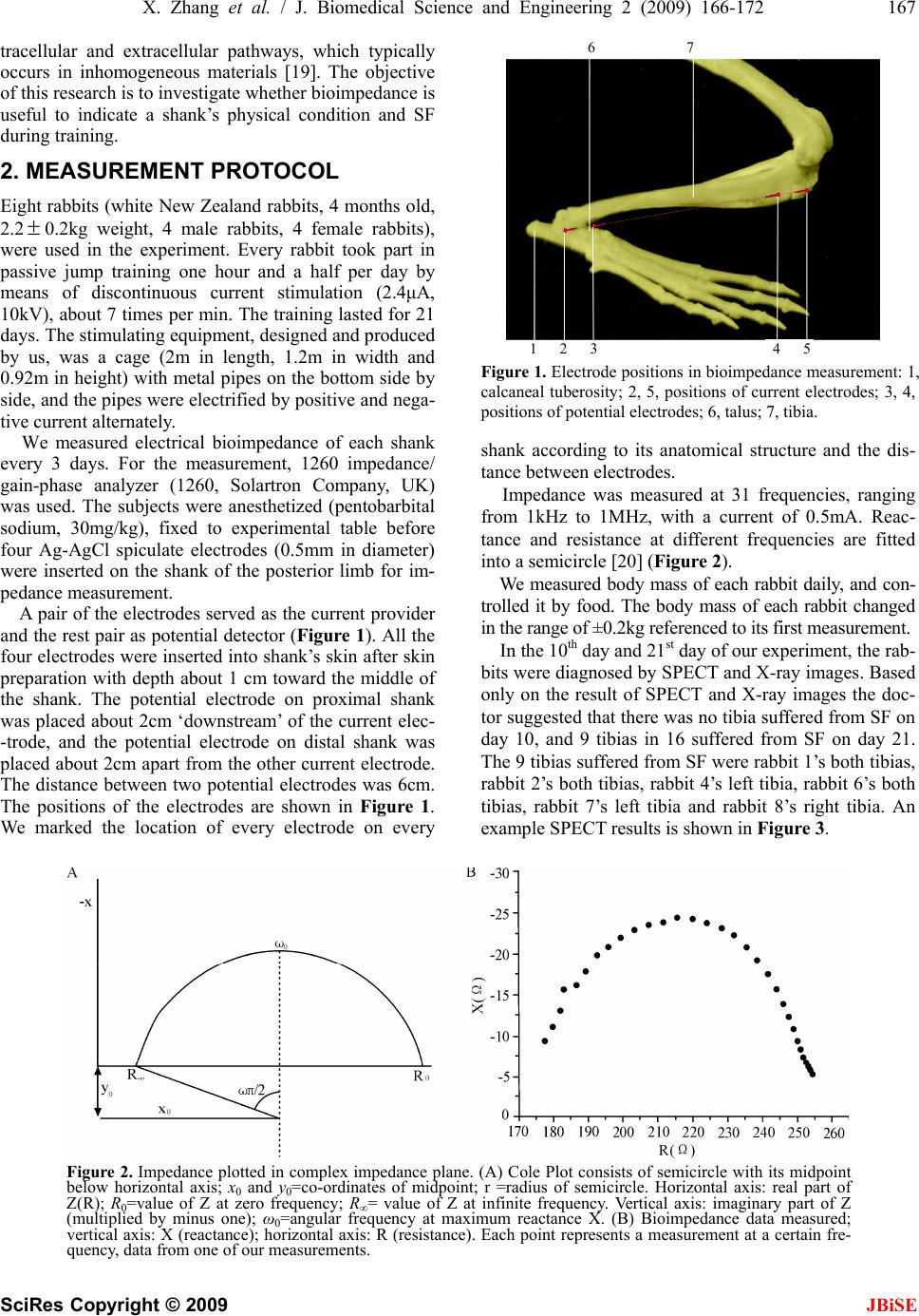 X. Zhang et al. / J. Biomedical Science and Engineering 2 (2009) 166-172 167 SciRes Copyright © 2009 JBiSE tracellular and extracellular pathways, which typically occurs in inhomogeneous materials [19]. The objective of this research is to investigate whether bioimpedance is useful to indicate a shank’s physical condition and SF during training. 2. MEASUREMENT PROTOCOL Eight rabbits (white New Zealand rabbits, 4 months old, 2.2 0.2kg weight, 4 male rabbits, 4 female rabbits), were used in the experiment. Every rabbit took part in passive jump training one hour and a half per day by means of discontinuous current stimulation (2.4μA, 10kV), about 7 times per min. The training lasted for 21 days. The stimulating equipment, designed and produced by us, was a cage (2m in length, 1.2m in width and 0.92m in height) with metal pipes on the bottom side by side, and the pipes were electrified by positive and nega- tive current alternately. We measured electrical bioimpedance of each shank every 3 days. For the measurement, 1260 impedance/ gain-phase analyzer (1260, Solartron Company, UK) was used. The subjects were anesthetized (pentobarbital sodium, 30mg/kg), fixed to experimental table before four Ag-AgCl spiculate electrodes (0.5mm in diameter) were inserted on the shank of the posterior limb for im- pedance measurement. A pair of the electrodes served as the current provider and the rest pair as potential detector (Figure 1). All the four electrodes were inserted into shank’s skin after skin preparation with depth about 1 cm toward the middle of the shank. The potential electrode on proximal shank was placed about 2cm ‘downstream’ of the current elec- -trode, and the potential electrode on distal shank was placed about 2cm apart from the other current electrode. The distance between two potential electrodes was 6cm. The positions of the electrodes are shown in Figure 1. We marked the location of every electrode on every 6 7 Figure 1. Electrode positions in bioimpedance measurement: 1, calcaneal tuberosity; 2, 5, positions of current electrodes; 3, 4, positions of potential electrodes; 6, talus; 7, tibia. shank according to its anatomical structure and the dis- tance between electrodes. Impedance was measured at 31 frequencies, ranging from 1kHz to 1MHz, with a current of 0.5mA. Reac- tance and resistance at different frequencies are fitted into a semicircle [20] (Figure 2). We measured body mass of each rabbit daily, and con- trolled it by food. The body mass of each rabbit changed in the range of ±0.2kg referenced to its first measurement. In the 10th day and 21st day of our experiment, the rab- bits were diagnosed by SPECT and X-ray images. Based only on the result of SPECT and X-ray images the doc- tor suggested that there was no tibia suffered from SF on day 10, and 9 tibias in 16 suffered from SF on day 21. The 9 tibias suffered from SF were rabbit 1’s both tibias, rabbit 2’s both tibias, rabbit 4’s left tibia, rabbit 6’s both tibias, rabbit 7’s left tibia and rabbit 8’s right tibia. An example SPECT results is shown in Figure 3. Figure 2. Impedance plotted in complex impedance plane. (A) Cole Plot consists of semicircle with its midpoint below horizontal axis; x0 and y0=co-ordinates of midpoint; r =radius of semicircle. Horizontal axis: real part of Z(R); R0=value of Z at zero frequency; R∞= value of Z at infinite frequency. Vertical axis: imaginary part of Z (multiplied by minus one); ω0=angular frequency at maximum reactance X. (B) Bioimpedance data measured; vertical axis: X (reactance); horizontal axis: R (resistance). Each point represents a measurement at a certain fre- quency, data from one of our measurements. 1 2 34 5 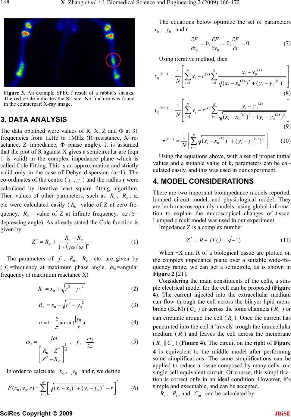 168 X. Zhang et al. / J. Biomedical Science and Engineering 2 (2009) 166-172 SciRes Copyright © 2009 JBiSE Figure 3. An example SPECT result of a rabbit’s shanks. The red circle indicates the SF site. No fracture was found in the counterpart X-ray image. 3. DATA ANALYSIS The data obtained were values of R, X, Z and Φ at 31 frequencies from 1kHz to 1MHz (R=resistance, X=re- actance, Z=impedance, Φ=phase angle). It is assumed that the plot of R against X gives a semicircular arc (eqn 1 is valid) in the complex impedance plane which is called Cole Fitting. This is an approximation and strictly valid only in the case of Debye dispersion (α=1). The co-ordinates of the centre (,) and the radius r were calculated by iterative least square fitting algorithm. Then values of other parameters, such as , , α, etc were calculated easily (=value of Z at zero fre- quency, = value of Z at infinite frequency, = depressing angle). As already stated the Cole function is given by 0 x 0 R 0 y 0 R R / R2 0 0 * /1 j RR RZ (1) The parameters of , , , etc. are given by (0=frequency at maximum phase angle, 0 f0 R R f0 =angular frequency at maximum reactance X) 2 0 2 00 yrxR (2) 2 0 2 0yrxR (3) )arcsin( 2 10 r y (4) 1 * * 0 0 RZ ZR j, 2 0 0f (5) In order to calculate , and r, we define 0 x0 y 2 1 2 0 2 000 )()(),,( N i ii ryyxxryxF (6) The equations below optimize the set of parameters , and r 0 x0 y 0,0,0 00 r F y F x F (7) Using iterative method, then N i N ik i k i k i k i k yyxx xx rx N x 11 2 )( 0 2 )( 0 )( 0 )( )1( 0 )()( 1 (8) N i N ik i k i k i k i k yyxx yy ry N y 11 2 )( 0 2 )( 0 )( 0 )( )1( 0 )()( 1 (9) N i k i k i kyyxx N r 0 2 )( 0 2 )( 0 )1( )()( 1 (10) Using the equations above, with a set of proper initial values and a suitable value of k, parameters can be cal- culated easily, and this was used in our experiment. 4. MODEL CONSIDERATIONS There are two important bioimpedance models reported, lumped circuit model, and physiological model. They are both macroscopically models, using global informa- tion to explain the microscopical changes of tissue. Lumped circuit model was used in our experiment. Impedance Z is a complex number )1( * jjXRZ (11) When -X and R of a biological tissue are plotted on the complex impedance plane over a suitable wide-fre- quency range, we can get a semicircle, as is shown in Figure 2 [21]. Considering the main constituents of the cells, a sim- ple electrical model for the cell can be proposed (Figure 4). The current injected into the extracellular medium can flow through the cell across the bilayer lipid mem- brane (BLM) () or across the ionic channels () or can circulate around the cell (). Once the current has penetrated into the cell it 'travels' trough the intracellular medium () and leaves the cell across the membrane (|| ) (Figure 4). The circuit on the right of Figure 4 is equivalent to the middle model after performing some simplifications. The same simplifications can be applied to reduce a tissue composed by many cells to a single cell equivalent circuit. Of course, this simplifica- tion is correct only in an ideal condition. However, it’s simple and executable, and can be accepted. m Cm R e R i R m Rm C e R, , and can be calculated by i Rm C 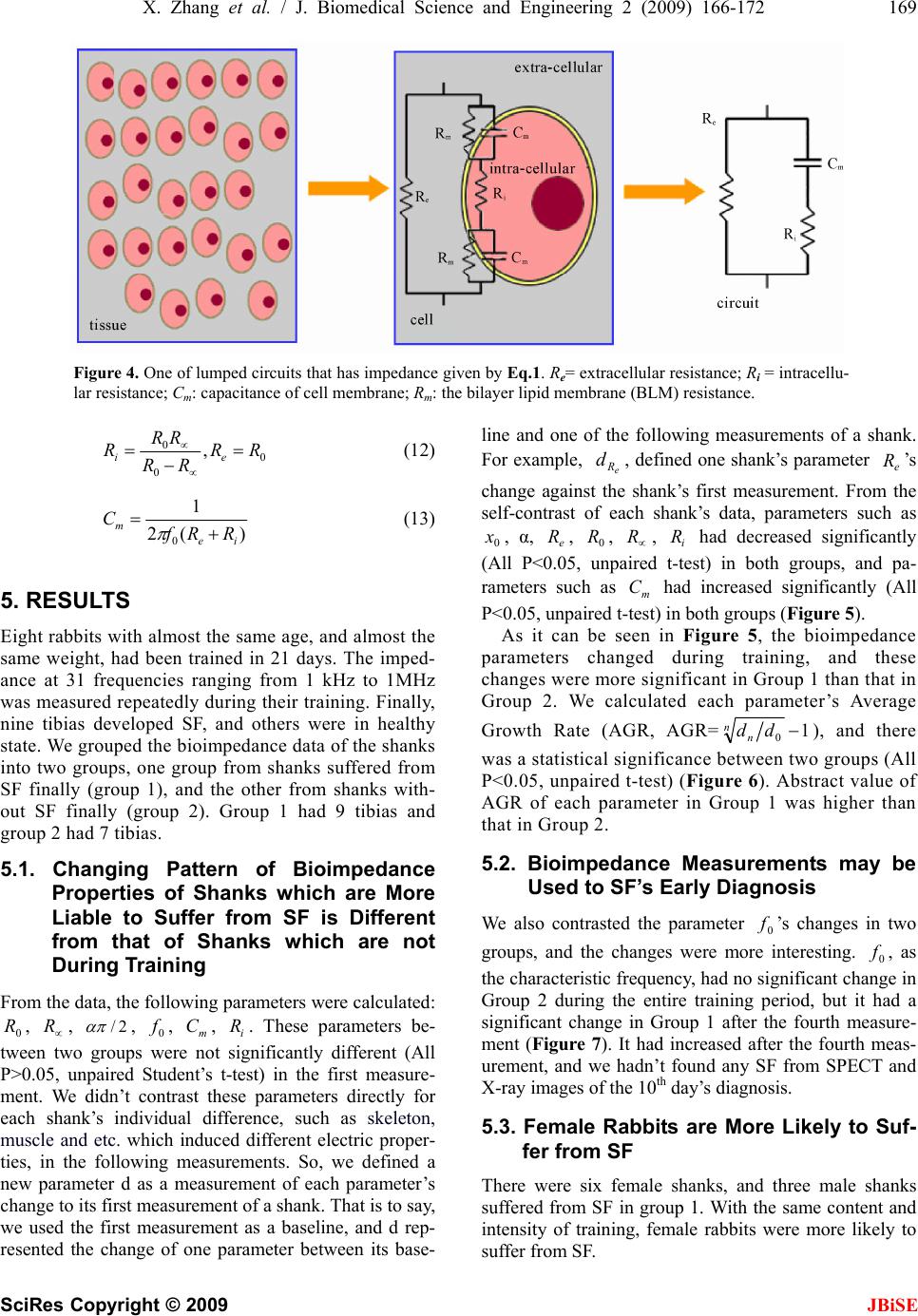 X. Zhang et al. / J. Biomedical Science and Engineering 2 (2009) 166-172 169 SciRes Copyright © 2009 Figure 4. One of lumped circuits that has impedance given by Eq.1. Re= extracellular resistance; Ri = intracellu- lar resistance; Cm: capacitance of cell membrane; Rm: the bilayer lipid membrane (BLM) resistance. 0 0 0,RR RR RR Rei (12) )(2 1 0ie mRRf C (13) 5. RESULTS JBiSE Eight rabbits with almost the same age, and almost the same weight, had been trained in 21 days. The imped- ance at 31 frequencies ranging from 1 kHz to 1MHz was measured repeatedly during their training. Finally, nine tibias developed SF, and others were in healthy state. We grouped the bioimpedance data of the shanks into two groups, one group from shanks suffered from SF finally (group 1), and the other from shanks with- out SF finally (group 2). Group 1 had 9 tibias and group 2 had 7 tibias. 5.1. Changing Pattern of Bioimpedance Properties of Shanks which are More Liable to Suffer from SF is Different from that of Shanks which are not During Training From the data, the following parameters were calculated: , , 0 R R2/ , , , . These parameters be- tween two groups were not significantly different (All P>0.05, unpaired Student’s t-test) in the first measure- ment. We didn’t contrast these parameters directly for each shank’s individual difference, such as skeleton, muscle and etc. which induced different electric proper- ties, in the following measurements. So, we defined a new parameter d as a measurement of each parameter’s change to its first measurement of a shank. That is to say, we used the first measurement as a baseline, and d rep- resented the change of one parameter between its base- line and one of the following measurements of a shank. For example, , defined one shank’s parameter ’s change against the shank’s first measurement. From the self-contrast of each shank’s data, parameters such as , α, , , , had decreased significantly (All P<0.05, unpaired t-test) in both groups, and pa- rameters such as had increased significantly (All P<0.05, unpaired t-test) in both groups (Figure 5). 0 fm Ci R e R d 0 R e R 0 xe R R m C i R As it can be seen in Figure 5, the bioimpedance parameters changed during training, and these changes were more significant in Group 1 than that in Group 2. We calculated each parameter’s Average Growth Rate (AGR, AGR=1 0 nndd ), and there was a statistical significance between two groups (All P<0.05, unpaired t-test) (Figure 6). Abstract value of AGR of each parameter in Group 1 was higher than that in Group 2. 5.2. Bioimpedance Measurements may be Used to SF’s Early Diagnosis We also contrasted the parameter ’s changes in two groups, and the changes were more interesting. , as the characteristic frequency, had no significant change in Group 2 during the entire training period, but it had a significant change in Group 1 after the fourth measure- ment (Figure 7). It had increased after the fourth meas- urement, and we hadn’t found any SF from SPECT and X-ray images of the 10th day’s diagnosis. 0 f 0 f 5.3. Female Rabbits are More Likely to Suf- fer from SF There were six female shanks, and three male shanks suffered from SF in group 1. With the same content and intensity of training, female rabbits were more likely to suffer from SF. 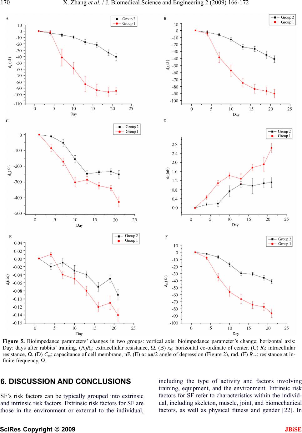 170 X. Zhang et al. / J. Biomedical Science and Engineering 2 (2009) 166-172 SciRes Copyright © 2009 JBiSE Figure 5. Bioimpedance parameters’ changes in two groups: vertical axis: bioimpedance parameter’s change; horizontal axis: Day: days after rabbits’ training. (A)Re: extracellular resistance, Ω. (B) x0: horizontal co-ordinate of center. (C) Ri: intracellular resistance, Ω. (D) Cm: capacitance of cell membrane, nF. (E) α: απ/2 angle of depression (Figure 2), rad. (F) R ∝ : resistance at in- finite frequency, Ω. 6. DISCUSSION AND CONCLUSIONS SF’s risk factors can be typically grouped into extrinsic and intrinsic risk factors. Extrinsic risk factors for SF are those in the environment or external to the individual, including the type of activity and factors involving training, equipment, and the environment. Intrinsic risk factors for SF refer to characteristics within the individ- ual, including skeleton, muscle, joint, and biomechanical factors, as well as physical fitness and gender [22]. In 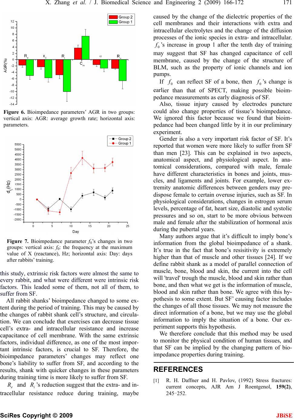 X. Zhang et al. / J. Biomedical Science and Engineering 2 (2009) 166-172 171 SciRes Copyright © 2009 JBiSE Figure 6. Bioimpedance parameters’ AGR in two groups: vertical axis: AGR: average growth rate; horizontal axis: parameters. Figure 7. Bioimpedance parameter f0’s changes in two groups: vertical axis: f0: the frequency at the maximum value of X (reactance), Hz; horizontal axis: Day: days after rabbits’ training. this study, extrinsic risk factors were almost the same to every rabbit, and what were different were intrinsic risk factors. This leaded some of them, not all of them, to suffer from SF. All rabbit shanks’ bioimpedance changed to some ex- tent during the period of training. This may be caused by the changes of rabbit shank cell’s structure, and circula- tion. We can conclude that exercises can decrease tissue cell’s extra- and intracellular resistance and increase capacitance of cell membrane. With the same extrinsic factors, individual difference, as one of the most impor- tant intrinsic factors, is crucial to SF. Therefore, the bioimpedance parameters’ changes may reflect one bone’s liability to suffer from SF, and according to the results, shank with quicker changes in these parameters during training time is more likely to suffer from SF. e R and ’s reduction suggest that the extra- and in- tracellular resistance reduce during training, maybe caused by the change of the dielectric properties of the cell membranes and their interactions with extra and intracellular electrolytes and the change of the diffusion processes of the ionic species in extra- and intracellular. ’s increase in group 1 after the tenth day of training may suggest that SF has changed capacitance of cell membrane, caused by the change of the structure of BLM, such as the property of ionic channels and ion pumps. i R 0 f If can reflect SF of a bone, then ’s change is earlier than that of SPECT, making possible bioim- pedance measurements as early diagnosis of SF. 0 f0 f Also, tissue injury caused by electrodes puncture could also change properties of tissue’s bioimpedance. We ignored this factor because we found that bioim- pedance had been changed little by it in our preliminary experiment. Gender is also a very important risk factor of SF. It’s reported that women were more likely to suffer from SF than men [23]. This can be explained in two aspects, anatomical aspect, and physiological aspect. In ana- tomical considerations, compared with male, female have different characteristics in bones and joints, mus- cles, and ligaments and joints. For example, lower ex- tremity anatomic differences between genders may pre- dispose female to certain overuse injuries, such as SF. In physiological considerations, changes in estrogen serum levels, percentage of fat, heart size, diastolic and systolic pressures and so on, start to be more obvious between male and female after the stabilization of hormonal axis during the pubertal years. Many authors argue that it’s difficult to imply bone’s information from the global bioimpedance of a shank. It’s true in the fact that bone’s resisitivity is extremely higher than that of muscle and other tissues [24]. If we define rabbit shank as a model of parallel connection of muscle, bone, blood and skin, the current into the cell will 'travel' trough the muscle, blood and skin rather than bone, and then what we get is the information of muscle, blood and skin rather than bone. We agree with this hy- pothesis to some extent. But SF’ causing factor includes the changes of all those tissues. We may not measure the direct information of a bone, but we may use the global information to imply the situation of a bone. Our ex- periment supports this hypothesis. We therefore conclude that this method may be used to monitor the physical condition of human tissues, and that SF can be implied by the changing pattern of bio- impedance properties during training. REFERENCES [1] R. H. Daffner and H. Pavlov, (1992) Stress fractures: current concepts, AJR Am J Roentgenol, 159(2), 245-252.  172 X. Zhang et al. / J. Biomedical Science and Engineering 2 (2009) 166-172 SciRes Copyright © 2009 JBiSE [2] R. L. Pentecost, R. A. Murray, and H. H. Bridley, (1964) Fatigue, insufficiency, and pathologic fractures, JAMA, 28(187), 1001- 1004. [3] M. Giladi, C. Milgrom, A. Simkin, and Y. Danon, (1991) Stress fractures: Identifiable risk factors, Am J Sports Med, 19(6), 647-652. [4] M. J. Kiuru, H. K. Pihlajamaki, and J. A. Ahovuo, (2004) Bone stress injuries, Acta Radiol, 45(3), 317-326. [5] M. Murcia, M. D., R. E. Brennan, M. D., and J. Edeiken, M. D., (1982) Computed tomography of stress fracture, Skeletal Radiol, 8, 193-195. [6] A. D. Perron, W. J. Brady, T. A. Keats, (2001) Principles of stress fracture management: The whys and hows of an increasingly common injury, Postgrad Med, 110(3), 115-8, 123-4. [7] M. T. Reeder, B. H. Dick, J. K. Atkins, A. B. Pribis, J. M. Martinez, (1996) Stress fractures: current concepts of di- agnosis and treatment, Sports Med, 22(3), 198-212. [8] L. M. Fayad, S. Kawamoto, I. R. Kamel, D. A. Bluemke, J. Eng, F. J. Frassica, and E. K. Fishman, (2005) Distinc- tion of long bone stress fractures from pathologic frac- tures on cross-sectional imaging: How successful are we? AJR Am J Roentgenol, 185(4), 915-924. [9] A. Feydy, J. Drapé, E. Beret, L. Sarazin, E. Pessis, A. Minoui, A. Chevrot, (1998) Longitudinal stress fractures of the tibia: Comparative study of CT and MR imaging, Eur Radio, 8(4), 598-602. [10] M. Gaeta, F. Minutoli, E. Scribano, G. Ascenti, S. Vinci, D. Bruschetta, L. Magaudda, A. Blandino, (2005) CT and MR imaging findings in athletes with early tibial stress injuries: comparison with bone scintigraphy findings and emphasis on cortical abnormalities, Radiology, 235(2), 553-561. [11] I. Elias, A. C. Zoga, S. M. Raikin, J. R. Peterson, M. P. Besser, W. B. Morrison, and M. E. Schweitzer, (2008) Bone stress injury of the ankle in professional ballet dancers seen on MRI, BMC Musculoskelet Disord, 9(1), 39, Published online, March 28, 2008. [12] M. W. Anderson and A. Greenspan, (1996) Stress frac- tures, Radiology, 199(1), 1-12. [13] A. Fottner and C. Birkenmaier, (2008) Stress fractures presenting as tumours: A retrospective analysis of 22 cases: Reply to Agarwal and Gulati, Int Orthop, Pub- lished online, August 6, 2008. [14] D. Pauleit, T. Sommer, J. Textor, S. Flacke, C. Hasan, K. Steuer, D. Emous, and H. Schild, (1999) MRI diagnosis in longitudinal stress fractures: Differential diagnosis of Ewing sarcoma, Rofo, 170(1), 28-34. [15] S. T. Zwas, R. Elkanovitch, and G. Frank, (1987) Inter- pretation and classification of bone scintigraphic findings in stress fractures, J Nucl Med, 28(4), 452-457. [16] A. Thomasset, (1962) Bioelectrical properties of tissue impedance, Lyon Medical, 207, 107-118. [17] J. R. Bourne (ed.), J. -P. Morucci, M. E. Valentinuzzi, B. Rigaud, C. J. Felice, N. Chauveau, and P. M. Marsili, (1996) Bioelectrical impedance techniques in medicine, Critical Reviews in Biomedical Engineering, 24(4-6). [18] H. P. Schwan, (1957) Electrical properties of tissue and cell suspensions, Adv Biol Med Phys, 5, 147-209. [19] B. Rigaud, L. Hamzaoui, N. Chauveau, M. Granie, J. -P. Scotto D. Rinaldi, and J. -P. Morucci, (1994) Tissue characterization by impedance: a multifrequency ap- proach, Physiol Meas, 15, A13- A20. [20] K. S. Cole, (1940) Permeability and impermeability of cell membranes for ions, Cold Spring Harbor Symp Quant Biol, 8, 110-122. [21] E. T. Mcadams and J. Jossinet, (1996) Problems in equivalent circuit modelling of the electrical properties of biological tissues, Bioelectrochem, Bioenergetics, 40, 147-152. [22] S. J. Warden, D. B. Burr, and P. D. Brukner, (2006) Stress fractures: Pathophysiology, epidemiology, and risk fac- tors, Current Osteoporosis Reports, Published online, March 26, 2008. [23] A. Ivković, M. Franić, I. Bojanić, and M. Pećina, (2007) Overuse injuries in female athletes, Croat Med J, 48(6), 767-778. [24] T. J. C. Faes, H. A. van der Meij, J. C. de Munck, and R. M. Heethaar, (1999) The electric resistivity of human tissues (100Hz–10MHz): A meta-analysis of review studies, Physiol Meas, 20, R1-R10.
|