Open Journal of Social Sciences, 2014, 2, 1-5
Published Online March 2014 in SciRes. http://www.scir p.org/journal/jss
http://dx.doi.org/10.4236/jss.2014.23001
How to cite this paper: Lin, J. and Sung, J. (2014) Assessing the Graham’s Formula for Stock Selection: Too Good to Be True?
Open Journal of Social Sciences, 2, 1-5. http://dx.doi.org/10.4236/jss.2014.23001
Assessing the Graham’s Formula for Stock
Selection: Too Good to Be True?
Jason Lin1, Jane Sung2
1Depart men t of Business Administration, Tr uma n State University, Kirksville, US A
2Depart men t of Econo mics, Tr uma n State Univers ity, Kirksvi lle, USA
Email: jlin@truman.edu
Received Oct ob er 2013
Abstract
Benjamin G r ah am o ffered a str aig h tfo rw ard and simple formula to evalu ate sto cks’ in trinsic value.
Many r e g ard the G r ah am Formula is a very sim plist ic w ay of me asur ing an in divid ual comp any’s
intrinsic value. Gr aham a nd War re n Buffe t ho weve r felt tha t the simp lici ty of the mod el allowed
them to quickly an d ac cu r atel y id entify undervalued companies, and s ta y aw ay f ro m over valu ed
ones. In this p ap er, we wa nted to explore the ef fectivenes s of th e G raham ’ s formula. We wan ted to
see if using the Gr aham ’s formula, investors c an ac hieve excess retu rn s abo v e the ma rke t over a
period of 17 years.
Keywords
Graham’s Formula; Intrinsic Value
1. Introduction
Many regard the Graham Formula is a very simplistic way of measuring an individual company’s intrinsic value.
Graham and Warren Buf fet howeve r felt that the simplicit y of the model allowed them to qui ckly and accurately
identify und erval ued companies, and sta y away from overvalued ones. They unders t ood that other stra tegie s
could produc e excess retur ns , but t hat this strategy allowed t hem to do so with les s r i sk. T he formula was origi-
nally developed by economist Benjamin Graham in 1962 and was fur ther revised by Mr. Graham in 1974 [1].
The fo rmula requires two company specific inputs and one systematic inp ut . The two company specific inputs
are the co mpany’s earnings p er share for the past twelve months and t he co mpany’s long-term ear ning s g rowth
estimate. The one syste matic input is the yield on AAA corporate bonds. This allo ws the investor to take into
account economic conditions that change the r isk premium for low risk bonds, and the specific earnings and t he
growth of these e a rnin gs. Althou gh us ua l ly described as the fa ther of value i nvestin g, the formul a can mor e ac-
curately be described as G.A.R.P. or growth at a reasonable price because the higher t he growth the more value
the fo rmu la at trib utes to the sto ck.
While many view this method as far too simplistic to pred ict minor fluct uatio ns in the market, the Gr aham
Formula has b een proven to be extremely useful in anal yzing the s to ck marke t crash in October 1987. A study in
the May-Ju ne 1988 Harvard Business Review titled “The Smart Crash of October 19th”, the author s of the study,
J. Lin, J. Sung
2
Arbel , Car vell, a nd P ostnieks, (1988) [2] showed ho w re markably well the Graham formula worked. The study
showe d that nearly all the stocks on the market were overvalued on October 1, 1987, usi ng the Relati ve Graham
Value (intrinsic value using Graham For mu l a divided by the curre nt sto ck price). Duri ng the period preceding
the crash many in the inve s t ing c ommunity talked about how t he Graham formu la was outda ted and inconsist ent
with ratio nal prices of the day. Ho wever, when the markets closed on October 19, 1987, the Relat ive Graham
Value wa s r e markably close to one for a large majority of stocks lis ted on t he excha nge (Arbel, 1988). [2] The
authors believed that instead of a burst of irrationality, the crash was a return to rationalit y when investors rea-
lized they couldn’t make p r ofits by buying overvalued se curities and sell in g them at a higher price because
eventually no one would pay that amount. D uring this period, t he Graham formula was ve ry accurate in predict-
ing stock prices and the authors believe this is evidence that the Graham formul a is a good tool for assi gnin g
value to a company’s stock.
The authors of the study hypothesized that as the cr ash was ha ppe ni ng, many investors went back to a funda-
mental approach of stock valuation, rat her than the irr atio nal exuberance that typified the 1980s stock market.
Thi s was made clear by the fact that a valuation techniq ue suc h as the Graham Formula was so us eful in ex-
plaining why stocks fell to the level they did. If the Graham formu la was a good predictor of stock price, it
wo u ld work best whe n markets were rational a nd there was no mispricing d ue to an over exuberance as the au-
thor s believed the re was preceding the crash.
In this paper, we want ed to explore the effectiveness of the Graham’s for m u la. We wa n te d to se e if using the
Graham’s formula, investors can ac hieve excess returns above the market over a period of 17 years.
2. Literature Review
The G raham for mu la is a product of the 1930’s market cra s h, and coming from those uncertain times, its goal
was to “stand the test of the ever enigmatic futureas Graham himself mentioned in the preface to his book
“Security Anal yst ” [3]. Graham developed his theor y and elaborated on it in two of his mos t famous books,
“Security Analyst” and “The Intelligent In vestor”. T he main concept behind the formula is the b e lie f that co m-
panies have an intrinsic value whi ch the market doesn’t necessarily reflect in their st o ck prices. The intrin sic
value includes both tangible and intan gible p ar ts of the co mpany and its de termination is based on fundamen tal
analysis rather than the stock price. Investor s houldn’t be too concerned with the s hort ter m fluc t uati ons in stock
price, rather they should focus on the long run in order to achieve excess returns.
Benjamin Graha m offered a straightforward a nd simple formula to evaluate stocks’ intri nsic va l ue. T he for-
mula consists of four inputs: current earnings per share, projected growth, the underlying appropriate earnings
yield and i nterest expectations based on the AAA corporate bonds. This si mplic it y of the formula is in stark
contrast to today’s complex models, and perhaps because of its simplicity, it’s often ignored in valuati on me-
thods and dis mis sed as too naive.
Using Graham’s formula, a Relative Graham Value ( RGV) is calc ulated by dividing the stock’s i ntrin sic val-
ue by its current price [2]. It can be used to analyze whether a stock is under value d or ove rvalue d. If the RGV is
above one, according to this theory the stock is under value d and thus a good buy. On the contrary, if the RGV is
belo w one the sto ck is ove rva l ued and thus a good sell. The idea behind the Graham’s formula howeve r, goe s
against developments in more recent fina ncial the ory, most notably the efficient market hypothesis. Whereas the
followers of the ef ficie nt market hypothesis belie ve t ha t the market incorporates any new infor matio n int o the
stock prices, proponents of Graham arg ue that this is not the case. Using t he Graham’s formula, they belie ve that
stoc ks can be underpriced and overpriced by the market and as such, there exist opportunities for re turns in
excess of the market. Most notable investors t hat follow Benjamin Graham’s philosophy are Warren Buffett,
Jo hn Bogle a nd Mario Gabelli. The ideas of Graham are not mainstrea m however , and as stated earlier, many
dismiss the formula at to o simple and not so p histica ted e nough.
3. Data and Methodology
To assess the predictive value of Graham’s formula, we us ed t he stock p ric e a nd EPS of the 30 Blue C hi p com-
J. Lin, J. Sung
3
panies that compose the Dow Jones ind e x [4]. The rule that we followed was tha t if the sto ck reached a RGV
over our predetermined criterion, it wo u ld be bought and if the RGV we n t belo w it, it wo u l d be sold. Several
assumptions were u se d in findi ng the input va lues for the Graham formulas:
1) The time period used in the comparison went from 1997 until 2013.
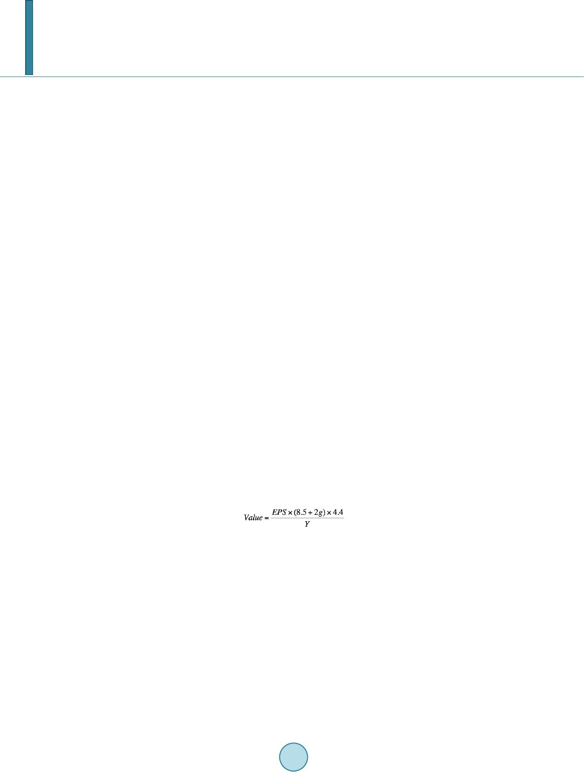
2) Diluted EPS of the 30 blue c hi p stocks was used.
3) Growth rate used was the annualized growth in EPS over the pr evious five years; to prevent negative stock
prices, we li mited t he growth factor to 4.25% which would make 8.5 + 2 g = 0.
4) For corpor a te bond rates, we used an nualized yield based on monthly bond yields.
5) Stock prices and Dow Jones data were taken from the adj usted close on J une 30th each year or the nearest
previous tr ad in g day; further more stocks were ad justed fo r stoc k splits.
6) We checked to see if we needed to buy or sell stocks only on June 30th.
7) As the Do w Jo ne s has changed c omposition, we followe d suit; we o nly invested in sto cks that were in the
composite as of June 30thand divested of stocks that left the composite.
Furthermore , our anal ysis wa s split in two separate trials wit h RGV le vels of 1.25 and 1.50 respectively. We
bought the stock wh en its RG V was above the level and so ld it when the RGV went bel o w one. The por tfolio
was composed of equal market value s of every stock invested in at the beginning of each year. Fina l ly, for the
purpose of this portfolio we liq uida ted o ur positions in 2013 regardless of the RGV.
We attempted to remove all sources of survivor ship b ias by usi ng t he curre nt Dow Jo nes component compa-
nies for each year. We were able to find most of the companies still exist in one form or another b ut two stocks’
data were har d to come by, AT & T before the merger with SB C and Union Carbide. In both of these cases, the
company became a wholly owned subsid iary of another company and t here is no currently traded stock that re-
flects thei r historical prices.
4. Results
Our findings related to Graham’s formula’s predictive power are quite remarkable. As stated b efore, we wanted
to know whether or not Gra ham’s formula coul d be used to achieve excess returns above the market as an in-
vesto r. Benjamin Graham wa s a proponent of taking co nsiderable margin of sa fet y in investment decisions to
allow for error in analysis and to provide for a str onger a rgument in favor of the same inve s tment decisio n
(Graham, 2006) [1]. Fo r this reason, we assumed a position in the companies with RGV’s greater tha n o ne at
two different margins of safety levels. An RGV above one s ugges ts tha t the company is currently underpriced in
the mark et and shoul d be bo ught, whereas an RGV below 1 suggests t hat the company is overvalued. W ith this
in mind and to t e st t he strength of Graham’s formula, we assu med a portfolio that purchased i nt o companies
whe never their RGV wa s above one by a margin of safety of 25% and 50% (two separa te trials) and sold the
company’s securities whe never their RGV fe ll belo w one. We felt that pur cha si ng and se lli ng at these respective
levels was the best way to test the predictive power of Graham’s for m ula because that is what it implied-an
RGV above one means t he company’s stock is undervalued and an RGV below one means the company is
overval ued. A gain, what we f ound was p re tt y impressive.
If, startin g before 1997, you selected companies to invest in based solely on Graham’s formula and held the
criteria that t he companies mus t be trading at an RGV below one wi th a margin of safety of at 25%, you would
have o utperformed the Do w Jones Indust rial Average in every year from 1997 to 2013 except for thre e years
(1998, 2003, and 2011). The following Table 1 shows our resul ts wi th t he firs t column be i ng how much excess
return Graham’s formul a was able to generate above the Dow Jones Industr i al Average each year. The second
column is measuring year over year, how much did the Graham’s over perform the market on a cumulative ba si s.
In the years that Graham’s formula underperformed the market, it only underperformed marginall y. Whe n Gr a-
ham’s formula over performed the market, however, it did so substantially as we can see by 2013, the cumula-
tive over p erformance by Graham’s formu la was 119.44% over the seve nteen years.
For the portfolio where we took considerably more margin of safety at 50%, the results were even better.
Graham’s formul a performed better t han the DJIA in every single year. The second ha l f of the Ta bl e 1 summa-
rizes our r e s ul ts for holding this portfolio. This phe nome nal track record leads to the cu mulative r eturn over t he
DJIA in our second p or tfolio to be substantial l y higher, almo st double that of our first portfolio.
If we look at the ret urns as a year over year compounded effect on total returns, we can see the difference in a
measurable dollar amount. From 1997 to 2013, the Dow Jones Ind ustr i al Ave rage went from 7672 to 14,975. If
J. Lin, J. Sung
4
Table 1. Summery of portfolio returns.
Case I Case II
Buy at RGV >= 1.25 Buy at RGV >= 1.5
Return over DJIA Cumulative Return Return over DJIA Cumulative Return
1998 1.57% 1.57% 0.21% 0.21%
1999 4.95% 3.30% 5.05% 5.27%
2000 6.15% 9.66% 6.15% 11.74%
2001 19.95% 31.53% 22.05% 36.38%
2002 2.95% 35.41% 4.91% 43.08%
2003 1.90% 32.84% 4.34% 49.29%
2004 6.71% 41.75% 19.47% 78.38%
2005 10.15% 56.14% 18.51% 111.37%
2006 3.05% 60.90% 6.74% 125.62%
2007 1.91% 63.98% 1.57% 129.16%
2008 7.01% 75.47% 6.94% 145.06%
2009 9.21% 91.63% 10.14% 169.91%
2010 5.21% 101.62% 6.15% 186.51%
2011 1.64% 98.31% 1.47% 190.72%
2012 4.95% 108.13% 6.21% 208.78%
2013 5.44% 119.44% 6.95% 230.24%
we investe d the amount of the DJIA index level ($7672) in 1997 in our portfolio guided by Graham’s for m u la
and purchased securities wit h RGV’s greater tha n or equal to 1.25 while selling them when b elow 1, would end
up as $32,861.14 at the end of June, 2013. If we invested $7672 in our portfolio as guided by Graham’s formula
and purchase d securities wit h an RG V greater t han or equal to 1.5 while selling them when below 1, our $7672
wo u ld be worth $49453.44 at the end of June, 2013. Bear in mind that t his excludes any transaction costs asso-
ciated with buying and selling as dictated by Graham’s formula or fees associated with holding a mutual/index
fund to mimic the DJI A portfolio. This is al s o under the assu mptio n that our po r tfolio can only be revisited once
per year, meani ng we c heck the RG V level of our sec uritie s o nly on June 30 th of each year . Thi s means that our
securities could be meeting our sell criterion so metime dur ing the year before or after June 30th, and we would
not have sold. The opposite case is also true-somet ime during the year before or after Ju ne 30th the stock c oul d
have been meeting our buy criterion but we would not have bought. This represents a ver y illiquid portfolio
whi ch onl y a dj us t s its securities based on annual re-eval uati on. It would ha ve been interes tin g to see if Graham’s
formula could have outperformed or even underperformed the market more so if we allowed for monthly or
even daily re-evaluati on.
5. Conclud ing Remark s
We find Graham’s formula mystifying in wa y s . One of the most simple valuatio n methods that we have ever
seen produced by one of the most int ellige nt a nd di stinguished minds in the hist ory of finance. Even though t he
data that was pr esented to you suggests tha t Graham’s formula can be actively used to outperform the marke t
given a suf ficie nt margin of safety, we are still hesitant moving forward to use this method as investo rs because
of how worr yi ngl y simple it is. The formula does not ask for much and thus you’ re left fee ling that you will not
get much in return either. We feel this could be one of the ma in unde rl yi ng reasons for the formula’ s succe ss.
No matter the evidence you present in favor of its predictive abilities, it likely is not used much if at all by insti-
J. Lin, J. Sung
5
tutional investors because of it perceived naivety. This could give t he user of the formula an advantage. The
market, a collection of all investors, determines stock price s at any given point in time. If thi s formula was used
on a large scale by many inve s t ors t he pr o ba bility of outperforming the market woul d have to d ec line as prices
reflect Graham’s intrinsic value. Gi ven tha t Graham’s formula ha s b een successful in retrospect and its usage is
likely limited, this could provide potential for indi vi dual investors to do well in the markets. For those of us who
do not have eno ugh time to e ngage in individual sec urity analysis and to keep up with the market, Graham’s
formula provides hope. Over t he p a st se venteen years, using Graham’s formula could ha ve netted an investor
more t han double, in dollar amounts, what the Do w Jone s I ndustria l Average would have netted them. Historical
performance is never an i ndicato r of futur e performance, but we have compelling evidence to suggest that there
is so me stren gth in this formula. Combined with furt he r analysis and multiple o t he r analy ses the formul a could
provide an individua l investo rs appreciable returns and ease of mind.
References
[1] Arbel, A., Carvell, S. and Postnieks, E. (1988) The Smart Crash of October 19th. Harvard Business Review, 124-136.
[2] Ben jamin, G. (2013) Investopedia. http://www.investopedia.com/terms/b/bengraham.asp
[3] Graham, B. (2006) The Intelligent Investor. Harper, New York.
[4] Morningstar (2013) Morningstar Articles RSS.