Advances in Historical Studies
2014. Vol.3, No.1, 22-32
Published Online February 2014 in SciRes (http://www.scirp.org/journal/ahs) http://dx.doi.org/10.4236/ahs.2014.31004
Open Access 22
A Tentative Interpretation of the Epistemological Significance
of the Encrypted Message Sent by Newton to Leibniz
in October 1676
Jean G. Dhombres
Centre Alexandre Koyré-Ecole des Hautes Etudes en Sciences Sociales, Paris, France
Received October 8th, 2013; revised November 9th, 2013; accepted November 16th, 2013
Copyright © 2014 Jean G. Dhombres. This is an open access article distributed under the Creative Commons
Attribution License, which permits unrestricted use, distribution, and reproduction in any medium, provided the
original work is properly cited. In accordance of the Creative Commons Attribution License all Copyrights ©
2014 are reserved for SCIRP and the owner of the intellectual property Jean G. Dhombres. All Copyright ©
2014 are guarded by law and by SCIRP as a guardian.
In Principia mathematica philosophiæ naturalis (1687), with regard to binomial formula and so general
Calculus, Newton claimed that Leibniz proposed a similar procedure. As usual within Newtonian style, no
explanation was provided on that, and nowadays it could only be decoded by Newton himself. In fact to
the point, not even he gave up any mention of Leibniz in 1726 on the occasion of the third edition of the
Principia. In this research, I analyse this controversy comparing the encrypted passages, and I will show
that at least two ideas were proposed: vice versa and the algebraic handing of series.
Keywords: Leibniz; Newton; Calculus Principia; Binomial Series; Controversy; Vice Versa
Introduction
In a conference devoted to resentment seen as an object for
the historian, I tried to account for the vindictive attitude that
Newton gradually developed towards Leibniz. What is pro-
found in the quarrel was not really about who first discovered a
path to Calculus, but how one happens to recognize a revolu-
tionary theory in mathematics has been prepared with the req-
uisites of rigour accepted at a certain time. And more, it is to
know how it is possible to ensure that a new theory is actually
completed. I then necessarily reduced my presentation of
mathematical facts, emphasizing only on the perception of an
innovator in science, who may imagine accordingly that any
other creator was to succeed only by following the same path1.
Resentment may then arise from the almost experimental rec-
ognition that this almost automatic thought is not true. Public
sources on the so-called priority quarrel between Newton and
Leibniz, which began in 1699 through the fault of Nicolas Fatio
de Duillier, are numerous enough to afford such a psychologi-
cal study2. But more can be said, outside any theory of emo-
tions. Here I am to focus on a purely epistemological aspect,
restricting even to a specific expression, precisely the one given
by what is called the epistola posterior. The name was coined
by Newton himself to refer to the second letter he wrote in Oc-
tober 1676 to Leibniz. In it Newton explained that he had a
method for dealing with “quantities” (not yet said variable but
flowing3), when related by an equation, and that there was a
double reciprocal link between these quantities and their speed
of change, called fluxions4. Newton wrote about a “vice versa”
procedure (Figure 1). It has always been thought that this
meant the relation between differential and integral calculus5.
Newton mingled the procedure, so is his precise verb, with the
way to handle series algebraically. I just quote the memoran-
dum found in Newton’s papers, but give translation of the two
deciphered parts only.
My paper confronts the fact that the meaning of what was
encrypted, which included at least two ideas (one is the vice
versa and the other is the algebraic handing of series), could
only be decoded by Newton himself. In his famous Principia
mathematica philosophiæ naturalis in 1687, eleven years later,
Newton claimed that Leibniz had a similar procedure, but there he
did not explain the vice versa. I am not sure, contrary to what
Hall was thinking, that this attitude of Newton helped to clarify
1Voir Jean Dhombres, is it interesting to qualify as resentment some epi-
sodes of the priority quarrel between Leibniz and Newton? Reflexions on
pyschological aspects in history of science, Geneva colloquium of October
2012 on Resentment, under the responsability of Dolorès Martín Moruno, to
appear.
2See: Rupert Hall, 1980; Koyré, 1968; Newton, 1999; Whiteside, 1960;
Whiteside (ed.), 1967-1974; Guicciardini, 1998; Panza, 2005; Harper, 2011;
Dhombres, forthcoming 1.
3The expression for a variable was invented by de L’Hôpital in
A
nalyse des
infiniment petits, a book published in 1696 at the Imprimerie royale in Paris.
The expression “to flow” was sometimes used in Latin by Cavalieri in 1635,
to describe the move of a straight line through a given geometric figure.
4The vocabulary for fluxions was settled in Newton’s manuscripts around
1671, but was used earlier around 1666, which is by the way only ten years
before 1676.
5Remark that this common thought is based on the idea that computation
with fluxions and its inverse, which is obtaining fluents from fluxions, is
exactly the same as differential and integral calculus. That this idea was the
principle on which a biased judgment of the Royal Society had been found-
ed against Leibniz in the early 18th century should prevent us from accepting
it without any further discussion.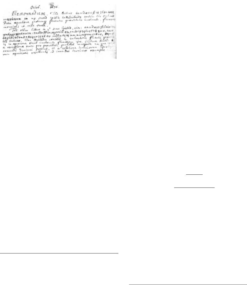

J. G. DHOMBRES
Open Access 23
1. Given an equation involving any number of fluent quantities to fin
d
the fluxions and vice versa.
2. One method consists in extracting a fluent quantity from an equation
at the same time involving its fluxion; but another by assuming a series
for any unknown quantity whatever, from which the rest could con-
veniently be derived, and in collecting homologous terms of the resul-
ting equation in order to elicit the terms of the assumed series
6
.
Figure 1.
Translations of Newton’s Memorandum possibly from October1676, as
it is dated, where he deciphered the two encrypted messages he sent to
Leibniz.
his relationship to Leibniz7. To the point he gave up any men-
tion of Leibniz in 1726 on the occasion of the third edition of
the Principia. If my basic assumption is that Leibniz could
absolutely not decipher these messages8, and Newton knew it
beforehand, I make a second assumption for the present pres-
entation. Newton would think that at least part of the non en-
crypted content of the letter, the one devoted to the now-called
Newton’s binomial, would have been enough for Leibniz to
grasp the meaning of “vice versa”. The link with series, bino-
mial series in fact, has always been considered by historians as
basic to the understanding of Newton’s ways. In other words, to
conduct the present study, I am assuming that Newton thought
he had invented calculus of fluxions and its inverse on the basis
of a meditation on the binomial theorem. Or, better said, New-
ton thought this meditation on the binomial formula provided
the only reasonable access to the new Calculus. So that what is
in the epistola posterior in reference to the binomial theorem
should be sufficient to rebuild his inventive steps.
An Outline
The question is now to see how such a thesis can be docu-
mented. In what may also be seen as a reconstruction of New-
ton possible epistemological feelings9, I use some documents in
addition to this second letter that I will not comment in more
details10. But I selected few other documents, and in fact only
three authors will help me. First, Nicolaus Mercator, of whom
John Wallis presented a paper to the Philosophical Transac-
tions in 1668. It is generally acknowledged that this paper made
an impression on Newton; he even might have thought that his
deepest and unpublished thoughts had been discovered. So my
purpose is to check from Newton’s second letter what could
have been analogous in Mercator’s Logarithmotechnia. On the
other hand, I will quote Gregory of Saint-Vincent11, as his name
appeared in a note by Christiaan Huygens for the Académie
royale des science the same year 1668, when he precisely com-
mented Mercator’s results, and wanted to give a more balanced
history than the one essentially based on Wallis that Mercator
had provided.
But before going to this year 1668, when absolutely nothing
about fluxions had been known outside Newton, I have to make
clear, at least from our actual point of view, what precisely
binomial formula could teach. It seems to me that this way,
perhaps even because of its anachronistic position, helps under-
standing the past. The only condition is to always confront with
what we know about the available knowledge in the past, as
discussed by the available historiography. So history of science
has to engage not only a confrontation between two periods of
time, but with the tradition as well.
What the Binomial Formula May Provide about
Newton’s Vice Versa Formulation?
Newton’s Binomial formula is the development in power se-
ries of a given power of a binomial, generally written nowadays
as (1 + x), the power being α
, in fact any number:
() ()
()( )
2
1
11 2!
11
!
n
xx x
nx
n
α
αα
α
αα α
+
+=+++
−−+
++



(1)
This formula has a finite number of terms when exponent α
is an integer, thus providing what is called Pascal’s triangle.
Except that coefficients in (1) are analyzed, while in Pascal’s
triangle they are computed through an iterative construction.
The second member of (1) is an infinite series for all other val-
ues of α
, even when 1 α =− , and this particular case will
play a leading role. The binomial series may be considered as a
definition of an exponential, and so is the case by Cauchy in his
1821 Cours d’Analyse algébrique, for which it was necessary
to consider limitations on values of x, so that to ensure conver-
gence of the series (in fact the modulus of x, or its absolute
value if one restricts to real values, should be strictly less than
1). In 1676, nobody except Gregory of Saint-Vincent had pro-
vided a definition of an exponential when an irrational expo-
nent α
was at stake. Newton’s formulation of the binomial
was explicitly restricted to rational exponents, and even in this
6This memorandum is in the “waste-
b
ook” kept in the University Library o
f
Cambridge (Add. 4004, fol. 81v), and with the help of Newton it was al-
ready printed by Wallis for the third volume of his Mathematical works
where he put a Latin translation of his Treatise on algebra (1693). The deci-
pherment also appeared in the Commercium Epistolicum in 1712.
7Hall, 1980.
8By the way, some letters are missing in the second coding, see Turnbull,
1960, p. 159.
9I am using this terminology in order to avoid a contemporary tendency to
reduce epistemology to logic and to an analytic side, thus destroying what
Gaston Bachelard analyzed so carefully, under the name of “obstacle épis-
témologique”. Very roughly speaking, it is a process of thought by which
something cannot be discovered or even expressed because common views
prevent any investigation on this side. Kuhn modified this idea with the no-
tion of a paradigm, or model for normal science at a time, thus replacing
common views, but requiring an external object not fitting to the paradigm
and its logic, the explanation of which will then destroy normal science, to
get another one.
10The second letter of 1676 Newton intended for Leibniz through Oldenburg
acting as secretary of the Royal Society established ten years earlier, is
available in Latin and in an English translation in Turnbull (ed.), 1960, vol.
II, pp. 110-161. A French translation was given in the thesis of Michel Pen-
sivy, 1987. I am not analyzing the whole letter, and as in a stylistic exercise,
concentrate on the binomial formula only.
11Jesuit fathers usually named him by his first name, in Latin, Gregorius.
The name in French, Grégoire de Saint-Vincent, was not used at the time,
and in 1668 for the Paris Academy of science, Huygens used the form
Gregorius de Sancto Vincentio. I will use the form Gregory of Saint-Vin-
cent.

J. G. DHOMBRES
Open Access 24
case he did not attempt a proper definition. There has been
however an earlier use by Wallis with the square root of 3.
Let us integrate the left member of (1), under the restriction
1 α ≠− . One side gives an integration result,
() ()
1
0
11
1d 11
xx
tt
α
α
αα
+
+
+= −
++

and so we deduce by applying (1) in the case of exponent
1 α +, then dividing by 1 α +, and with the elimination of the
constant term:
()
()( )
2
01d 2!
12
!
x
n
ttx x
nx
n
α
α
αα α
+=++
−−+
++



(2)
From the second member of (1), we may compute in a dif-
ferent way, this time using formal integration term by term of
every power of x, and here there is a need for a more special-
ized integration result
1
0d1
n
xn
x
tt n
+
=+
.
By this process, the first member of (1) becomes the first
member of (2), and the second member of (1) becomes another
series, so that one has:
()
() () ()
2
01d 2
111
1
(1)!
x
n
x
ttx
nx
nn
α
α
αα α
+=++
−−−+
++
−



(3)
Fortunately the two second members of (2) and (3) are being
identical once rearranged. So that one sees then that the way
integration works for a xn or for ()
1
x
α
+, with the two formu-
las which were respectively used for the two previous ways
along with (1), is reflected in the way coefficients of the bino-
mial formula are behaving. But we will see that our writing of
coefficients is not the way Newton wrote about to Leibniz.
In the case 1 α =− , one starts from a well known particular
case,
()
2
111
1
nn
xx x
x=− +++−+ +

(1)’
This time however, one has not another binomial to use for
integration of the two members. One has to rely on a com-
pletely different situation, as the Neper logarithmic function ap-
pears.
() ()
23 1
ln 11
23
n
n
xx x
xx n
−
+=− + ++−+
(2)’
We get as well, when playing with variable x (in fact chang-
ing x into –x in the integration process)
23
1
ln 123
n
xx x
x
xn
=+++ ++
−

(3)’
This last result that may be visualized in the original paper
(see Figure 2) was the great novelty of Mercator’s Logarith-
motechnia12, which had been prepared a year before. In this
case attested in 1668, one sees that coefficients of the binomial
formula are well adapted to integration of powers of x.
Pay attention to the fact that I am not pretending here any-
thing about the way Newton could have obtained the binomial
formula13. He never proved it, even if this formula was essential
to his Methodus fluxionum, for which there is a well established
manuscript in 1671, and which was never published by New-
ton14 who died in 1727. What I will precisely be looking at is
the way Newton wrote binomial formula, in his October 1676
letter to Leibniz (via Oldenburg). We will see that Newton’s
writing reflects the behaviour of coefficients towards integra-
tion, using in fact various integration formula, form the simple
one for integer powers of x, even in the case of −1, or for any
power of x. I am then suggesting that conversely integration of
powers of x can be deduced from this specific writing of the
binomial formula, and then, precisely from the aspect of the
formula as a series, integration appears as well for any function
(supposedly represented by a power series).
So that I first have to provide Newton’s formulation, as it can
be read in Newton’s letter for the development of a binomial
with a rational exponent15 (m, and n, are integers, possibly neg-
ative, and not zero):
()
2
23
m
mn
nmmnmn
P PQPAQBQCQ
nn n
−−
+=++ ++
Some explanations are required. In fact, the first letter of the
alphabet A denotes the first term
m
n
P
to the right of the equal
sign. Newton wanted to have it so denoted so that B, the second
letter in the alphabet, appearing in the third term of the series,
denotes the second term m
A
Q
n. Then C as third letter of the
alphabet, appearing in the fourth term, is to denote the third
term, and so on. Modern terminology exhibits the same play on
coefficients with a displacement of a unit. I do not believe by
the way that I am modifying the significance of what Newton
did by putting index numbers where he used alphabetical order,
and even by taking P = 1 and Q = x. But I know what I am
inducing when I add a functional notation in order to state the
dependence of letter A in m
n (so that I write f1), or B (which I
write f2), C, and so on. By using a concept not present in New-
ton’s mind, I am trying to show as clearly as possible that
Newton’s binomial, as any exponential like y
x
, requires two
variables, one denoted by Newton as Q, and the other is the
exponent m
n. I may then replace Newton’s manner by a visible
dependence of coefficients, in order to obtain the formulation:
()
121
2
231
1
m
nmmm
xfff x
nnn
mmm
ff fx
nnn
 
+= +
 
 

++


12Mercator, 1668.
13Whiteside, 1961.
14It is generally said that Castillon is the first to have provided a proof in
1742 for Newton’s binomial formula, but in fact it appeared as early as 1708
in a textbook by Charles Reyneau, L’Analyse démontrée, with a new edition
in 1736 (See Jean Dhombres, forthcoming 2). There was also a proof in
F
luxionum Methodus Inversa by Cheyne in 1703.
15Newton did not use parenthesis for the binomial P + PQ, but he drew a
line above the whole binomial, ended by a descending vertical line.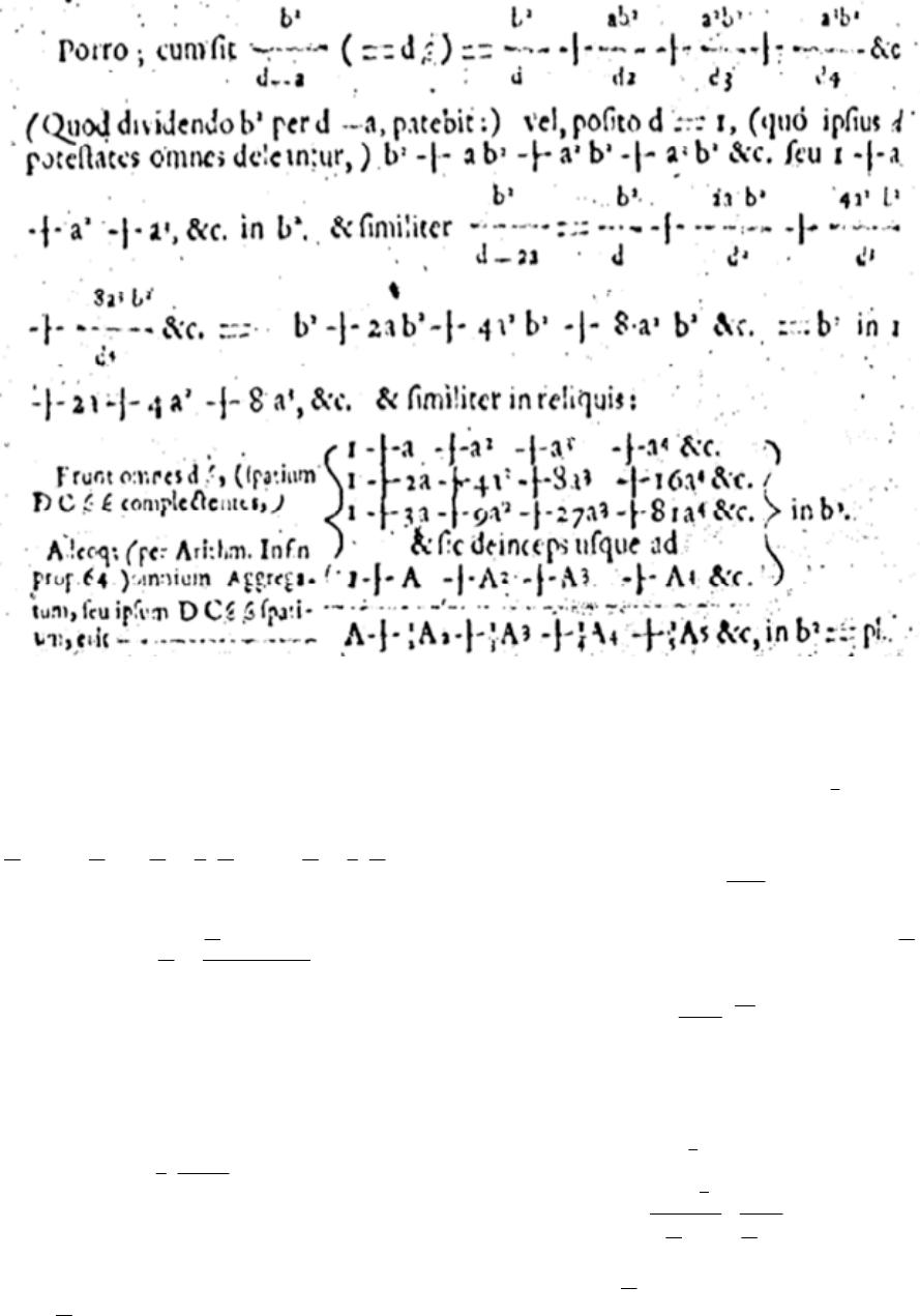

J. G. DHOMBRES
Open Access 25
Figure 2.
A page full of computations of series, taken from Mercator by Wallis, in his presentation to the Royal Society in August 1668, p. 758. At
the last line is the famous Logarithmic series (see relation (3)’), and the word quadrature is there forgotten as the abbreviation pl appears,
for plane area, which is interpreted as a logarithm, due to Gregory of Saint-Vincent’s result as stated by de Sarasa. This formula is very
efficient for small values of A, so that it avoids the lengthy computation of a whole table for logarithms.
I know from Newton’s writing that the final result will have
to be:
123 4
11
1,,1 ,2
23
mmmmmm
ffff
nnnnnn
 
==−=−
 
 
and more generally for
()
11
2, 1
k
mk
mn
kf
nk
−−+

≥=
 −
 .
In other words, these forms exhibit the very particular be-
haviour I am looking for, as there is a unit less taken at each
successive occurrence, and a division by an integer a unit fur-
ther. This is the form of the successive terms Newton chose to
exhibit with A, B, C, etc., without exhibiting m/n, but for exam-
ple in the form where one sees the place of successive integers
like 2 and 3 in
12
3
mn
n
−



.
So the general writing for coefficients as in (2), our common
way of writing, is not the generality that Newton was interested
in. For the use of Leibniz, he preferred to focus on the double
behaviour for integers. The proper gymnastic on the generality
of variable m
n, for which one has to add a unit (which corre-
sponds to the integration in x of power
()
1
m
n
x
+), is an integra-
tion that for xk divides it by k+1, and for
()
1
x
α
+ divides it by
1 α +. At the end, the combinatorial play lies on the formula
1
0
d1
x
x
tt
α
α
α
+
=+
,
the nature of which is more hidden if one uses m
n
α =, and
separates integers m and n in the form:
mn
n
n
x
mn
+
+,
which was the one used in Newton’s time.
Let me here add an excursus for how we may then determine
functions fk. If as Newton we leave undecided the values of
functions A, B, C, ⋅⋅⋅, if we consider as proven that the integra-
tion in variable x of
()
1
m
n
x
+ be
()
1
1
11
1
m
n
mm
n
x
n
+
+
−
+
+,
so avoiding case 10
m
n+= , and if we moreover accept to in-
tegrate a series term by term, according to Descartes’ undeter-

J. G. DHOMBRES
Open Access 26
mined coefficients method extended to power series in x, a
cascade of equalities is obtained. The presentation is being
facilitated by the numbering Newton had chosen, with the al-
phabetical order and his iterative writing with products. The
identity
23
121 21
12
1
3
1
2
32
111
11
23
1
1
1
1
1
11
1
1
m
mmmxmmmx
fxf ff f f
nnn nnn
fff
mm
mm m
nnn
nn n
mmm
mn
x
ff
n
fx
n
n
 
++ +
 
 
 
=− ++
 
 

+++
++
  
+
+
++ +


+
+


yields in fact 111
m
n
f =


+. It is here that the generality of the
computation on the variable must imply as well that
11fm
n

=

 .
The second equality yields,
21 1
111
1
mm m
mnn
ff
n
n
f

++
+

=


,
and by using what has been previously proved, we get
211fmm
nn

=


++
.
With the same procedure on the variable m
n, we deduce
2
fmm
nn

=

 .
The third equality is reduced to
2
11
2
11
1
mm m
mn
fnn
n

=

++


+
,
that is:
211
2
mm
nn
f =


+.
So we see precisely a unit less and division by an integer
having a unit more. So that
2
1
21
mm
nn
f −

=

  


.
The possibility of a solution leads in effect, and for
()
11
2, 1
k
mk
mn
kf
nk
−−+

≥=
 −
 .
I have doubts this last proof (that I named an excursus) could
have been thought by Newton. Not because there are techni-
calities unproved with the handling of series, but because the
core of the proof is the form of a function. As I went from x to x
+ 1, or perhaps more properly said, from m/n to (m + n)/n. I
think the idea of a function came only once integral calculus
was understood. I so have not used such changes on functions
for the proofs I gave concerning Newton’s writing of the bino-
mial formula and what one may deduce for integration theory16.
However, to the list I gave of presuppositions for the validity of
Newton’s show to Leibniz, I have to add that integration was
indeed supposed to be an additive process. Was it not what
Newton intended to explain by exhibiting precisely series, on
which he wrote in his memorandum? That the integration proc-
ess was additive could have been confirmed for Newton by the
very result Mercator had obtained with (2)’. Mercator was not
using a priori considerations on integration, playing precisely
with Riemann sums as we will see, from which the additive
property of integration on functions is obvious. We may also
think that Newton used what Cavalieri had shown earlier with
his very specific figures adding surfaces from addition of
lengths in his Geometria indivisibilibus, and other works on in-
divisibles. We also know that, at least for some integers, the
result
1
0d1
n
xn
x
tt n
+
=+

was important to Cavalieri.
Mercator’s Results as Presented to the Royal
Society and an Addition by Huygens
My second step is to check an earlier use of the binomial
formula and of power series17. As announced, I take the pres-
entation by Mercator in 1668, published in the issue of the Phi-
losophical Transactions dated Monday, 17th August 1668. The
brochure (Figure 3) gave two analysis of books done by John
Wallis, the latest being that of a Logarithmotechnia.
Wallis presented it in the form of a letter to Lord Viscount
Brouncker18, dated July 8 in Oxford. Brouncker had previously
worked on similar techniques on the hyperbola. So that this is a
good example on how the Royal Society worked, outside offi-
cial meetings using an active correspondence. There too is a
proof of a few pages in a second letter of Wallis dated August 8;
it had been specifically requested by Brouncker on August 3rd.
In this issue, there is an extract provided by Mercator himself of
his Logarithmotechnia. This book was appearing the same year
in London. All these texts are accompanied by two figures only,
by which Wallis attracted even more attention they resemble
figures found in his Arithmetica infinitorum, already twelve
years old (Figures 4 and 5).
If Wallis reported on the book, it is in part because there was
“an accurate and subtle construction of logarithms”. It is a nu-
merical display, and explains the reason why Mercator’s name
is famous. But it was also clear Mercator had a way of “squar-
ing of the hyperbole”19, as Wallis named it.
16However I considered it was then easy to deduce the integration between 0
and of x to power n from the primitive of a binomial with any power.
17I am not considering here the way James Gregory, in a letter dated 1670,
p
roved the binomial formula by using an interpolation. Recall that I am not
here in the quest for an archeology of the binomial formula, but looking at
the meaning Newton intended to give by presenting this formula to Leibniz,
where the encrypted messages are given.
18Quoting Lord Viscount Brouncker was relevant, as this member of the
Royal Society had published in the same third volume of the Philosophica
l
Transactions some results on The Squaring of the Hyperbola by an infinite
Series of rational Numbers (p. 645-649).
19The quotation in Latin is page 753 in the third volume of Philosophica
l
Transactions, and the reference made to Figure 1 is to the figure provided
with the figure here numbered as Figure 4.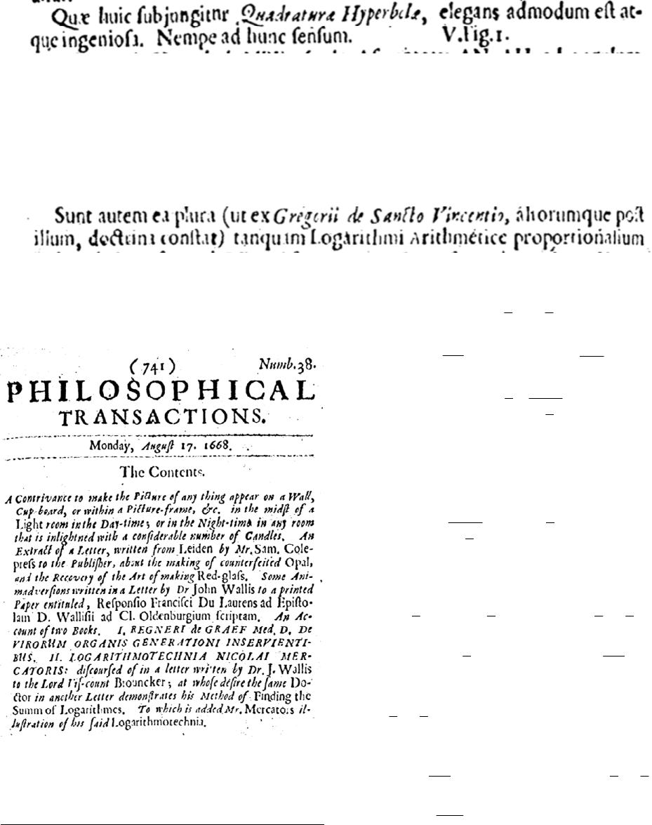

J. G. DHOMBRES
Open Access 27
Figure (a).
The word “quadrature” (see Figures (a) and (b)) lost a large
part of its meaning, in the sense that no square with an equal
area as the area of a hyperbolic segment is seen. Finding a se-
ries seems to be the new name for quadrature, but for sure
Leibniz and the Bernoulli brothers will give a different meaning
to quadrature, the one almost the same we use today when
speaking of different quadratures one has to achieve for differ-
ential equations. In fact, any mathematician of the time knew
that this was related to quadratures due to Gregory of Saint-
Vincent. This author was later quoted in the presentation by
Wallis. But few readers could find a link between this statement
on Gregory of Saint-Vincent and the paraphernalia of algebraic
formulas Mercator presented20.
Figure (b).
I think the following modern terminology will be enough to
understand Mercator’s computations (see Figure 2). I directly
start with “Riemann sums”21.
Figure 3.
The presentation page of the issue of the Philosophical Transactions
where Mercator’s ideas were presented, and at the end of this presenta-
tion, the announcement of the two figures about the “sum of Loga-
rithms”, which is just series (3)’.
()
1
0
n
nk
x
k
Sff x
nn
−
=

=


for the integral
0
d
1
xt
t+

, where I put
()
1
1
fx
x
=+. Then
()
1
0
1
1
n
nk
x
Sf k
n
x
n
−
=
=
+
.
These Riemann sums have equal steps, and this is precisely
such equal steps we see in Mercator’s figure with four parallel
lines (Figure 4). We also see such equal steps in Figure 5 by
Wallis. Binomial formula provides summation of the series
()
0
11
1
m
m
m
k
x
kn
x
n
∞
=

=−


+
,
and so we may write, using an inversion of the order of summa-
tion:
() () ()
() ()
11
00 00
111
1
1
000 0
11
1
11
mm
nn
mm
nkm mk
mnn
mm
nmm
m
mkm k
xk kx
Sfx x
nn nn
xkxk
nn
−∞∞ −
== ==
+
∞−∞ −
+
+
=== =
 
=− =−
 
 
 
=− =−
 
 
 
 
The last sum appearing is the Riemann sum, with equal
steps,
1
0
1m
n
k
k
nn
−
=



 which is related to the integral of xm be-
tween 0 and 1. So that when one goes to the limit in n,
() ()( )
1
1
00
0
1
0
d1
ln1lim1lim
1
1
m
xn
mm
n
nn
mk
m
m
tk
xSfx
tnn
x
m
∞−
+
→∞ →∞
==
+
∞
=

+=== −
+
=+



Outside convergence problems with inverting orders in sum-
mations and taking limits, questions, which shall not be treated
seriously before Cauchy and Gauss in the early 19th century, we
see that integration theory is taken by Mercator according to
two points of view. One is the numerical one, that is obtaining
20The quotation is page 758 in the third volume of Philosophical Transac-
tions.
21The anachronistic mention of Riemann sums to define integrals is useful to
understand how long it took to get a definition of integration different from
the simple inverse of derivation. But we know Riemann sums were used for
finding centres of gravity, volumes and for example in gauging methods for
ships.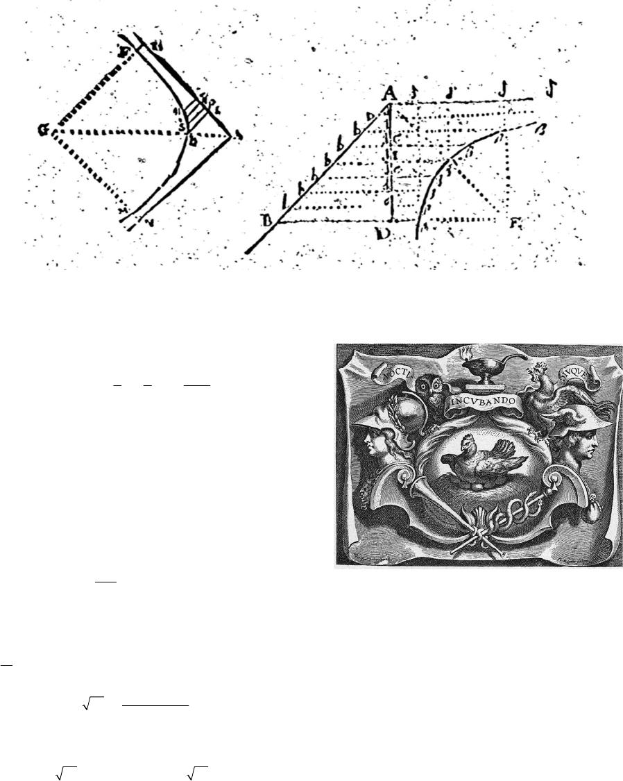

J. G. DHOMBRES
Open Access 28
Figures 4, 5.
The two figures published under n 38 in Philosophical Transactions for August 17th 1668 (this appears on page 756), the second
one being close to a figure in Arithmetica infinitorum (proposition XCV): one clearly sees parallel lines at equal intervals like in
many drawings on indivisibles, four parallel lines only in the first figure.
an integral by Riemann sums of constants steps, so that
11
0
0
11
dlim 1
m
n
m
nk
k
xx nnm
−
→∞ =


==



+



.
The last equality uses a result known for a long time in
Arithmetic (at least for small integers m), which precisely was
the main object in Wallis’ Arithmetica infinitorum, published in
1656. In place of an explicit limit, Wallis used a fraction with
an infinite number of terms, both for the numerator and the
denominator: he thus used an indeterminate integer n, having
first made a change of scale in the variable as well as on the
function. But this is not relevant for the present study.
The other integration theory used by Mercator is the loga-
rithmic result:
()
0
dln 1
1
xt
x
t=+ +
.
This had been found by Gregory of Saint-Vincent. More pre-
cisely the Flemish scientist had found that the variable area
under a hyperbola using an abscissa x, something we write now
as
()
1
d
xt
F
x
t=
, satisfies the relation:
()
() ()
2
Fa Fb
Fab + =.
In fact, Gregory expressed it geometrically by proving what
amounts to the following equality for areas:
()
() ()
()
Fab Fa FbFab−=−. (4)
This relation is not what Wallis and Mercator explicitly used
from Gregory of Saint-Vincent: as they considered there was
the expression of a logarithm (precisely because of (4)). These
conclusions had been expressed in 1649 by Antonio Alfonso de
Sarasa (see Figure 6 for a translation of this polemical title in
his book). He wrote under the guidance of Gregory of Saint-
Vincent, as may be checked form the manuscripts kept in the
In this proposition, two things are predicted by the person wh
o
claims it:
1. the proposition probably requires something far more dif-
ficult than the quadrature itself
2. squaring the circle by the Reverend Father Gregory of Saint-
Vincent loses itself in this still unsolved problem. By this, this
p
erson suggests that the solution to the problem of squaring th
e
circle will be released, if one overcomes the defect that was
indicated in the solution of the problem this person gave.
Author P. Alphonse Antoine de Sarasa from the Society of Jesus
Antwerp.
Figure 6.
Translation of the title of the booklet by de Sarasa in 1649,
where logarithms are identified with “hyperbolic spaces” and
associated vignette of the Plantin’s press, with an allegory on
meditation, as well as on financial difficulties to publish books.
Royal Library in Brussels (Mss. 5770-57793).
On the 17th of October 1668, only two months after the
presentation in London by Wallis and Mercator in the issue of
the Philosophical Transactions, Christiaan Huygens insisted in
a regular meeting of the Paris Academy of sciences on the true
origin of the computation involving logarithms. He even drew a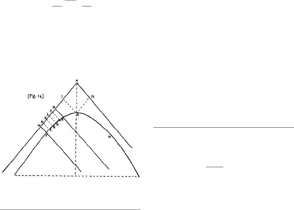

J. G. DHOMBRES
Open Access 29
figure (Figure 7) that is very similar to that of Mercator, and
provided a very short explanation (Figure 4).
Or cette dimension de l’hyperbole sert aussy a trouver les
logarithmes avec facilité parce que ces espaces hyper-
boliques comme VRHF, BIHF sont tousiours entre eulx
comme la raison de VR à FH est à la raison de BI a FH ce
que Gregorius de Sancto Vincentio a monstré le pre-
mier22.
Such a simple expression of the logarithmic property may
astonish the historian, but not the one who knows that Huygens
had truly discovered logarithms only some years before, and
had too corresponded with the then aged Gregory of Saint-
Vincent who explained to him his intellectual trajectory. In fact
Huygens was oversimplifying the expression of this mathema-
tician that we will have to study in our next step. This is also
frequent in history of mathematics: something that took years to
be understood, once published is viewed as obvious by a new
generation, or better said as new bases to build new things. For
the moment, it is enough to interpret this Huygens’ sentence in
our modern terminology, using the exponential notation but
keeping letters as organized in Figure 7, and adding pl in front
of VRHF just to mean the area of the “hyperbolic space” as was
named by Huygens, and to compare with Mercator’s writing.
plVRHF
plBIHF
BI VR
FH FH
 =


This amounts to what Gregory of Saint-Vincent had also
proved, as will be seen in my next step. Huygens immediately
transferred this result in “numerical” terms, and so forgot every
precaution about proportion theory. He made it clear that the
use of logarithms justified this direct way.
C’est a dire si l’on pose des nombres pour BI, VR, FH al-
ors comme l’espace VRHF est a BIHF ainsy sera la dif-
ference des logarithmes des nombres VR, FH a la differ-
Figure 7.
A figure used by Huygens at the Académie des sciences in Paris to
explain Mercator’s contribution presented in London two months ear-
lier.
ence des logarithms de BI, FH23.
Due to this maintenance of ratios for quantities as well as for
logarithms (therefore considered as numerical quantities), there
is no need here to specify the kind of logarithms being used.
That is any form like alnx + b will prove convenient. It is
enough in fact to have the functional property (4), a property
that was up to Mercator at the basis for the construction of
logarithmic tables.
Gregory of Saint-Vincent Methods for the
Logarithm and for the Exponential
My third step is to show how Gregory of Saint-Vincent
proved equality (4). He used Riemann sums, but with non equal
steps. In Figure 8, taken from Opus geometricum published in
1647, Gregory drew parallel lines forming rectangles (called
parallelograms in the written text) like FCX, MXG, etc. They
cannot be taken for “thick” indivisibles, in the sense that the
sizes measured by the abscissas are not uniform24. So that rec-
tangles with the same basis AH which are summed up in the
right part of the figure (Figure 8), would have to be put in de-
creasing values according to CX, XG, GI, IH, and so give more
than the error made by replacing the hyperbola FMELD by
rectangles named by three letters only, like FCX, MKG, etc. In
a similar but not exactly same way, rectangles appear in a fig-
ure (Figure 9) for a general curve in Newton’s Principia. One
may then pile up such rectangles aKbI, bLcm, etc., with the
same basis AB. The idea is to show how to pile up “small”
quantities, while keeping a “small” quantity. Smallness in this
figure is provided by length (Figure 9), as it is provided by
length CX (larger that XG, GI and IH in Figure 8). What is
surprising is that Newton kept unexplained a small rectangle
IfFB, drawn in part with dotted lines, which may precisely
show the fluxion of the area is the ordinate of the curve, a result
not at all mentioned in Gregory’s Opus geometricum.
Now I am ready for the fourth step, which is to read proposi-
tion 108 in Gregory of Saint-Vincent’s Opus geometricum. This
result is known as a quadrature of the hyperbola, but there is no
quadrature in the old sense, nor in the sense with series that
Mercator had used: an equality is obtained between a priori
numerically unknown areas.
Proposition 108: Let AB and AC be asymptotes to hyper-
bola DEF, and DH, EG and CF25 parallel26 to the asymp-
22This dimension of the hyperbola is also used to easily find logarithms as
hyperbolic spaces like VRHF and BIHF are always one to another as the
ratio of BI is to FH. This is what Gregory of Saint-Vincent was the first to
show. Huygens, 1668, p. 264.
23That is if one uses numbers for BI, VR, FH, then as space VRHF is to
B
IH
F
, so is the difference of logarithms of numbers VR and FH to the dif-
ference of logarithms of BI and FH. Huygens, 1668, p. 264. I have not
checked the original manuscript (Regi st res d e l’académie des sciences, tome
III, pp. 138-143), but I am using the very precise edition of the complete
works of Huygens (vol. 20, p. 261). Huygens’ sentence can be rendered in
the following terminology:
()
ln lnlnln
plVRHF
B
IFH VRFH
plBIHF −=−
.
24Cavalieri in 1635 drew parallel straight lines moving in such a way as to
cover entirely a figure, and so to generate an area. Such lines were called
indivisibles, and so they were supposed without any thickness. Thick indi-
visibles were later invented in order to link what Cavalieri did to what was
done on figures with Riemann sums, seen as geometric approximations to an
area.
25For analogy reasons, one should prefer the writing FC in this order. But
Gregory of Saint-Vincent chose quite often, in a sort of baroque mood, to
end a series of letters by inverting the order. As if to close something in the
appearance of a figure.
26The original text reads as “equidistant”.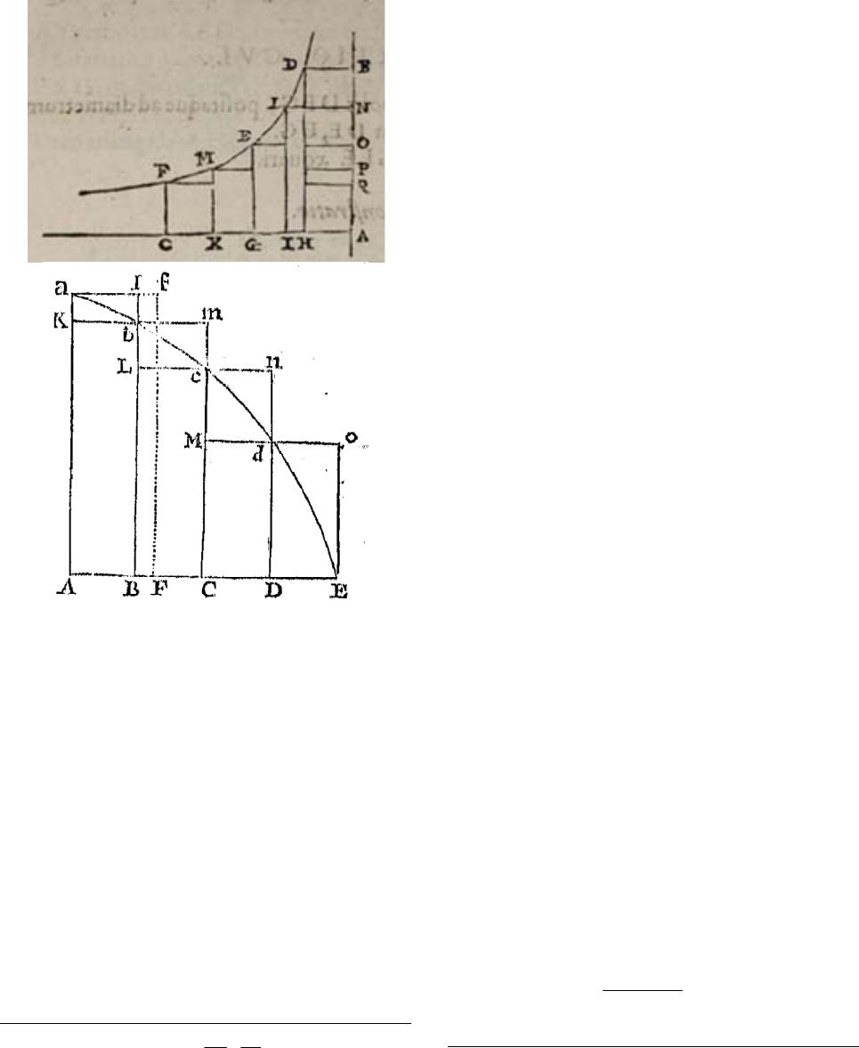

J. G. DHOMBRES
Open Access 30
Figures 8, 9.
Figure of a hyperbola accompanying proposition 108 in Book
VI of the Opus geometricum, published in Antwerpen in 1647.
The second figure is from Newton’s Principia. I chose the last
edition (1726, p. 28), which is here the same as in the original
1687 edition, to prove that Newton had not tried to modify the
way summation of infinitely small sums worked.
tote AB, be in continued proportion27. I say that segment
DHGE is equal to segment EGCF.
Its proof goes in the following way.
Proof: Let LI be given and put proportional means be-
tween HD MK, EG, CF, and draw BD, LN, EW, MP, FQ
parallel to the asymptote AC. Since DH, LI, EG, MK, FC,
continue the same ratio, AH, AI, AG, AK, CA, are propor-
tional28 (according to proposition 78 in this book). But
since the differences29 HI, GI, GK, etc., are proportional
(Proposition 1 of De progressionibus30) that HI is to IG,
AI is to AG, that is to say, as EG is to LI. This is why par-
allelograms LH and EI are equal. (by Proposition 14 of
this book). Also because GI is to GK as MK to EG, paral-
lelograms EI and MG are also equal. Similarly, parallelo-
gram FK is equal to parallelogram MG. So the four paral-
lelograms LH, EI, MG, FK are equal. So the two paral-
lelograms LH and EI cut off from segment EGHD are
equal to two parallelograms MG and FK cut off from
segment FCEG. Once again, if we set the mean propor-
tional between DH, LI31, EG, and between EG, MK, FC,
is shown in the same way as above, that the parallelo-
grams in segment EGHD are equal to the parallelograms
in segment FCEG. And since it can always be done in
such a way that the parallelograms cut off from segment
DHEG are greater than half segment DHEG and equal to
those who are cut off from segment EGFC are also larger
than the half of the same segment, it is clear that segment
FCEG is equal to segment EGDH (Proposition 116 of De
progressionibus). This was to be proved.
We notice that this is a direct procedure in this proof of an
equality. It is based on earlier and general proofs in the Opus
geometricum, put in book 2. It is related to what Newton will
do in 1687 under the name of ultimate ratios.
I am adding Figures 10 to 12 to show that Gregory of
Saint-Vincent’s procedure, but this time with parallel lines at
equal intervals, is used a second time in his book, at book 7, for
the ductus planum in plani. Such parallel lines appear as well in
Luca Valerio’s book on centers of gravity, in the early seven-
teenth century (Figure 13).
In book 6, to which we return, Gregory of Saint-Vincent
went further, and provided a figure (see Figure 14).
Proposition 129. Let AB32 and BC be asymptotes of the
hyperbola DFH, and let DE, FG, and HC33 be parallel to
the asymptote AB. Let plane surface FGCH be incom-
mensurable to plane surface DEGF. I say the ratio of DE
to FG multiplies the ratio of FG to HC as many times
quantity DEGF34 contains quantity FGCH (Dico rationem
DE ad FG, toties multiplicare rationem FG, ad HC, quo-
ties quantitas DECF, continet quantitatem FGCH)35.
Proposition 129 in the same book 6 on the hyperbola by
Gregory of Saint-Vincent gave the exponential property of
transforming a sum into a product. Gregory distinguished a
commensurable case (for which the reasoning by computation
is direct) and a non-commensurable case, easily proved by a
result of equality from Proposition 108. Gregory thus followed
the path chosen by Archimedes for his famous theory of the
lever in On planes equilibrium. His goal here was to define a
real number as an exponent, and as he has no name for it, he
called it a procedure of “many times”. It refers to what was
written earlier as a quotient of areas introduced by pl. This ex-
plains exponentiation, and is not restricted to rational exponents.
Gregory of Saint-Vincent thought in terms of numerical ratios.
It can be translated without betraying him by setting
areaDEGE
areaFGC H
α =,
and in a similar way,
27Continuous proportion just means: DH EG
EG CF
=.
28The hyperbola transforms a proportion on the abscissa-axis into one in the
ordinate-axis. The ratio of the proportion is reversed in the passage through
the hyperbola.
29The word difference is here to indicate a term like HI = AH − AI, to get a
continuous proportion as well.
30This is a reference to the second book in Opus geometricum.
31By mistake in the original text LE is written.
32A is missing in the figure, and should be read at the top left.
33This time, the last term HC is written by analogy with the three others.
34By mistake there is a C in place of a G.
35Gregory of Saint-Vincent used the same expression as in proposition 125,
but the “number of times” involved in the present proposition 129 is an
irrational number.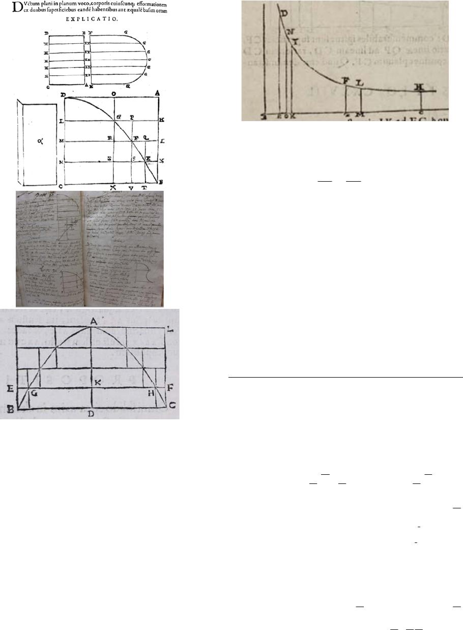

J. G. DHOMBRES
Open Access 31
Figures 10 to 13.
One of the first figure to the left in the book on ductus
by Gregory of Saint-Vincent, showing parallel lines at
equal intervals. It prepares an interpretation for solid
geometry. Therefore here there is no approximation
procedure. The next figure to the right appears in the
third chapter on the ductus, with a general “concave”
curve. It exhibits a way to prove that the sum of small
rectangles like GPFR, RFSN, etc., remains small as
being included in 0AEG, where EG gives a step for the
approximation. All letters are not clearly legible, and N,
for example, has been inverted by the printer. Next
figure is from a manuscript page with drawings from
what will become the seventh book on the ductus by
Gregory of Saint-Vincent, showing inscribed rectan-
gles for a general curve. One also sees a non concave
curve, and this generality is typical of this seventh
book of Opus geometricum. Last illustration is a figure
from De Cent r o g ravitati s due to Luca Valerio in 1606,
which certainly played a role in the scientific education
of Gregory of Saint-Vincent. One sees the approxima-
tion of the area of a parabola with circumscribed and
inscribed rectangles. The difference between these two
approximations is shown as an addition of small rec-
tangles, but they are not entirely piled up.
Figure 14.
Figure accompanying proposition 129 in the same book, with
parallel lines and no rectangles.
DE FG
FG HC
β

=

.
Therefore we have three possibilities only:
,, α
β
α
β
α
β
><=
. What is to be proved is that only the last
equality is true. It is enough to establish that the previous two
inequalities are false. Note that the functional property, which
is true for any exponential, is derived here from the geometric
evidence of addition of areas (one “sees”: xyx y aaa
+=). This
property of the exponentiation was not recognized at the time,
and almost never quoted by historians36. Thus it plays no role in
my present story. Except I wanted to show that a mathematician,
like Newton in this case, was not always able to see what was
important in another one, here Gregory of Saint-Vincent. So
that the hope that Leibniz could understand immediately his
mention of the binomial formula was certainly fallacious.
More than a Conclusion, and to Go Further
My conclusion indeed is that by the formulation Newton
36If exponentiation was really discovered and correctly defined by Gregory
of Saint-Vincent, it does not mean that he explained exponential of base e.
And so we may understand why Huygens chose to prefer using the already
constructed Neperian logarithm (without explicitly thinking it was the in-
verse of the exponential of base e). What is surprising is that Gregory had
everything to have the exponential of base e. A modern notation will make it
clear. Suppose that we take three points, named x1, x2 and x3, as abscissas
and corresponding y’s on the hyperbola (the Cartesian equation of which can
be written as xy = k). And denote by area 1, area 2, area 3, the successive
areas of the hyperbolic segments. What Gregory of Saint-Vincent proved in
proposition 129 is that:
area 2
area1
32
12
y y
yy
 =

 . If we define
1
area1
2
1
y
Ay

=
 , then we
have the expression of a ratio in terms of an exponential. That is area2 3
2
y
Ay =
In our modern way of writing, this just means that
1
k
eA
−
=. Gregory o
f
Saint-Vincent could have proved that his number
1
k
eA
−
= was not de-
pendent of the specific hyperbola used, or even have taken k = 1. He cer-
tainly could have proved, just form his result in Proposition 129 that what he
did with 1 and 2 to define Awould give the same number with 2 and 3, etc.
But he was not thinking in terms of a general representation of positive real
numbers (his general ratios) in terms of an exponential. Due to addition o
f
areas, he may see as well that area2area34
2
y
Ay
+=. And he may have, area3 4
3
y
Ay =
So that from the well known composition of ratios, 3
44
232
yyy
yyy
=, Gregory o
f
Saint-Vincent could have deduced the characteristic exponential property:
area1 area2area1area2
A
AA
+=.

J. G. DHOMBRES
Open Access 32
chose for the binomial he could think this was a good way to
exhibit to Leibniz the “vice versa”, that is the reciprocal link
between fluxional operation and integration operation, the two
being defined as independent operations. This was at least clear
in 1676, when Newton specifically insisted in writing this for-
mula by using a recurrence on coefficients and not an explicit
formula for such coefficients, later known as binomial coeffi-
cients. At this time, and after a long process, Newton had al-
ready obtained fluxions and integration, with separate defini-
tions. So that he then could be impressed by what he saw in the
binomial formula, quite independently of the fact that this for-
mula might have been as well at the beginning of his thoughts
on the Calculus. Another strong impression could be the fact
that what had been done with integration to understand the
recurrence for coefficients in the binomial formula, could be
done as well with derivation, this time using
()
()()
1
1
ddord11
nn
xnxx xx
αα
α
−
−
=+=+
or more properly said with the equivalence with dots in writing
fluxions37. This is important if we consider that for Newton,
following Leibniz, integration came first, and derivation after-
wards. At this time, year 1676, Newton might suppose that
Leibniz had obtained the same.
Later, textbooks on the Calculus began by explaining how
derivation or integration worked on powers of x, rational or
irrational, and so insisted far less on the binomial formula,
which appeared to be a formula of secondary importance. Such
textbooks, following Jean Bernoulli, were based on integration
as being defined as the inverse to derivation (so that the ap-
pearance of 1/n + 1 in the integration of xn was not a proof, but
the consequence of a definition and of derivation law). In this
way, textbooks forgot for a while Riemann sums and numerical
methods for approximation of areas or volumes. They however
were still used in practice. I warned at the outset that I certainly
was not trying here to decide between Leibniz and Newton on
the advantages and presentations of Calculus from derivation or
from integration: we all know that the differential notation is
better than the dots in the sense that a differential can be seen in
the writing of an integral, so clearly linking the two operations
to have one Calculus only. I so gave my basic assumptions
from the Newton memorandum. But I did not need to base my
account on an “innocence” of Newton, as I merely “see” what
one could get for the discovery of Calculus if Newton’s en-
crypted message was literally read. The advantage of my very
restrictive procedure is to avoid complicating the story with the
introduction of “indivisibles”, which Newton did not mention
in the text I chose. In May 1686, Leibniz felt the need to pre-
sent Cavalieri’s work as a start, or on his own terms, the “child-
hood of a resurgent science”38. This seems to contradict his
later presentation of integration as a mere inverse of derivation.
It was then a pleasure to give some place here to Gregory of
Saint-Vincent, as his importance lies in the fact that he speci-
fied integration as a process, inventing the notion of a primitive,
or indefinite integral. But, under the guidance of Huygens, I
associated the Flemish mathematician to Mercator, who pre-
ferred to mention Mersenne. This mathematician handled series
and algebraic notations, which Gregory of Saint-Vincent scorn-
ed or ignored and so could not go much further. Contrary to
Newton, as we have seen in his epistola posterior to Leibniz.
For my specific point of view here, it is the confluence of
two specific types of integration with different Riemann sums,
as we say today, which gave its numerical strength to Merca-
tor’s discovery. We must not forget that it caused a revolution
in the establishment of tables of logarithms. John Wallis had
only one type of integration due to his very specific notations
for Riemann sums with constant steps. It could have led to an-
other revolution in Newton’s mind, once he saw that the fluxion
of an area was precisely the function to be integrated. I have not
tried here to check what the information from Gregory of Saint-
Vincent and from Mercator could have brought to Leibniz, but
in the mind of the German mathematician, infinitesimals in
general played a major role, while we have seen Newton trying
to restrict to the integration process, then deducing the deriva-
tion process. There was a different way for Calculus, and the
Leibniz way was apparently the one privileged, outside applica-
tions of Calculus to various practical domains such that ships
stability, till Cauchy proved in 1821 the fundamental theorem
of Calculus showing that integration via Riemann sums indeed
corresponded to integration as inverse to derivation.
REFERENCES
Dhombres, J. (2014). Could or should Gregory of Saint-Vincent have
had to use indivisibles to present his own quadrature of the hyper-
bola that led to the logarithm and to the exponential? To appear in a
book by Birkhaüser Verlag, directed by Vincent Jullien, and entitled:
Indivisibles.
Dhombres, J. (2014). Les savoirs mathématiques et leurs pratiques
culturelles. Paris: Hermann.
Guicciardini, N. (1998). Did Newton use his calculus in the principia?
Centaurus, 40, 303-344.
http://dx.doi.org/10.1111/j.1600-0498.1998.tb00536.x
Harper, W. L. (2011). Isaac Newton’s scientific method. Oxford: Ox-
ford University Press.
Huygens, C. (1668). Sur la quadrature arithmétique de l’hyperbole par
Mercator et sur la méthode qui en résulte pour calculer les logarithms,
d’après les registres de l’académie pour le 17 octobre 1668. Oeuvres
de Huygens, 20, 261.
Koyré, A. (1968). Etudes newtoniennes. Paris: Gallimard.
Leibniz, G. W. (1686). De geometria recondita et analysi indivisibilium
atque infinitorum. Acta Eruditorum. In Math. Schriften, V, 228.
Mercator, N. (1668). Logarithmotechnia: Sive methodus construendi
Logarithmos, nova, accurate, & facilis, scripto antehàc communicata,
Anno Sc. 1667. Londres: Wilhelm Godbid.
Newton, I. (1999). The principia: Mathematical principles of natural
philosophy by Isaac Newton (translated by I. Bernard Cohen, Anne
Whitman). Berkeley: University of California Press.
Panza, M. (2005). Newton et l’origine de l’Analyse, 1664-1666. Paris:
Blanchard.
Pensivy, M. (1987). Jalons historiques pour une épistémologie de la
série infinie du binôme. Cahiers d’Histoire et de Philosophie des
sciences.
Rupert Hall, A. (1980). Philosophers at war. The quarrel between
Newton and Leibniz. Cambridge: Cambridge University Press.
http://dx.doi.org/10.1017/CBO9780511524066
Turnbull, H. W. (1960). The correspondance of Isaac Newton, Vol. II,
1676-1687. Cambridge: At the University Press.
Whiteside, D. T. (1960). Patterns of mathematical thought in the later
sevententh century. Archive for History of Exact Sciences, 1, 179-
388. http://dx.doi.org/10.1007/BF00327940
Whiteside, D. T. (1961). Newton’s discovery of the general binomial
theorem. Mathematical Gazette, 45, 175-180.
http://dx.doi.org/10.2307/3612767
Whiteside, D. T. (1967-1974). The mathematical papers of Isaac New-
ton. Cambridge: Cambridge University Press.
37This idea using derivation or fluxions is what seems to be claimed by
N
ewton in the exchanges in the priority quarrel. See Turnbull, 1960.
38Leibniz, 1686, p. 228.