 J. Biomedical Science and Engineering, 2009, 2, 136-143 Published Online June 2009 in SciRes. http://www.scirp.org/journal/jbise JBiSE Prediction of protein folding rates from primary sequence by fusing multiple sequential features Hong-Bin Shen1,3,*, Jiang-Ning Song2, Kuo-Chen Chou1,3 1Institute of Image Processing & Pattern Recognition, Shanghai Jiaotong University, 800 Dongchuan Road, Shanghai, 200240, China; 2Bioinformatics Center, Institute for Chemical Research, Kyoto University, Gokasho, Uji, Kyoto 611-0011, Japan; 3Gordon Life Sci- ence Institute, 13784 Torrey Del Mar Drive, San Diego, California 92130, USA. *Corresponding author: hbshen@sjtu.edu.cn Received 20 May 2009; revised 23 May 2009; accepted 1 June 2009. ABSTRACT We have developed a web-server for predicting the folding rate of a protein based on its amino acid sequence information alone. The web- server is called Pred-PFR (Predicting Protein Folding Rate). Pred-PFR is featured by fusing multiple individual predictors, each of which is established based on one special feat ure derived from the protein sequence. The ensemble pre- dictor thus formed is superior to the individual ones, as demonstrated by achieving higher correlation coefficient and lower root mean square deviation between the predicted and observed results when examined by the jack- knife cross-validation on a benchmark dataset constructed recently. As a user-friendly web- server, Pred-PFR is freely accessible to the public at www.csbio.sjtu.edu.cn/bioinf/Folding Rate/. Keywords: Protein Folding Rate; Ensemble Predictor; Fusion Approach; Web-Server; Pred-PFR 1. INTRODUCTION Knowledge of protein three-dimensional (3D) structures plays an indispensable role in molecular biology, cell biology, biomedicine, and drug design [1]. However, each protein begins as a polypeptide, translated from a sequence of mRNA as a linear chain of amino acids. A protein can function properly only if it is folded into a correct shape or conformation [2]. Failure to fold into the intended 3D structure usually produces inactive proteins with different properties. Although many efforts have been made trying to understand the mechanism of protein folding (see, e.g., [3,4,5,6]), it still remains one of the most challenging problems in molecular biology. In addition to understanding how a protein chain is folded, it is also important to find the folding rates of proteins from their primary sequences. Protein chains can fold into the functional 3D structures with quite dif- ferent rates, varying from several microseconds to even an hour [7,8]. Experimentally determining the three dimensional structure of a protein is often very difficult and expensive. However the sequence of that protein is easily known. Therefore, for quite a long time, scientists have tried to use the “least free energy principle” [2,9] to predict the 3D structures of proteins. Unfortunately, owing to the notorious local energy minimum problem, so far it can only be successfully used to address very limited structural characters, such as the handedness tendency and packing arrangement in proteins (see, e.g., [10,11,12]). In the past two decades, various statistical methods have been developed for predicting the struc- tural classes of proteins and their folding patterns ac- cording to the sequence information alone (see, e.g., [13,14,15,16,17,18,19,20,21,22,23,24,25,26,27,28] and a review [29]). Encouraged by the results obtained via these statistical approaches, various methods were de- veloped for predicting the folding rates of proteins be- cause the information thus acquired would be very use- ful for understanding the protein folding mechanism and the sequence-structure-function relationship [8,30]. In this regard, the approaches can be generally categorized into two groups: (1) the prediction of protein folding rates is based on the protein structure information; and (2) the prediction is based on the primary sequence in- formation. For the first group, the features of proteins are ex- tracted from their 3D structural information and hence the predictions are feasible only after the structures have been determined. Most of the methods in this group tried to derive the statistical significance of the correlation between the protein folding rate and the corresponding structural topological parameters, such as contact order (CO) [31], absolute contact order (Abs_CO) [32], total contact distance (TCD) [33], long-range order (LRO) [34], the fraction of local contact (FLC) [34], the chain  H. B. Shen et al. / J. Biomedical Science and Engineering 2 (2009) 136-143 137 SciRes Copyright © 2009 JBiSE topology parameter (CTP) [35] and the most recent geometric contact number (Nα) [30]. For the second group, the features of proteins are mainly extracted from their primary amino acid sequences, such as the amino acid biochemical properties [36] and the effective folding length (Leff) [8] derived from the se- quence-predicted secondary structure. The approaches in the second group are particularly useful when the 3D structural information of the protein concerned is not available. Although the aforementioned methods in predicting folding rates of proteins each have their own merits, they were all established by focusing on one (or a few) spe- cific feature(s). As is well known, a protein folding sys- tem is very complicated that involves many physical and chemical factors. For this kind of complicated biological system, it would be particularly effective to treat it by assembling many individual predictors with each oper- ated based on its own special feature [37,38]. In view of this, the present study was devoted to develop a novel ensemble predictor for predicting the folding rate of a protein chain by incorporating its many different fea- tures through an optimal fusion process. 2. MATERIALS AND METHODS To develop a powerful statistical predictor, the first im- portant thing is to obtain an effective benchmark dataset [39]. To realize this and also for facilitating comparison with the existing prediction methods, we use the bench- mark dataset as described below. 2.1. Benchmark Dataset The large dataset recently constructed by Ouyang and Liang [30] was used in the current study. It contains 80 proteins whose folding rates have been experimentally determined. Of the 80 proteins, 45 belong to the two- state folding behaviors without the visible intermediates while the other 35 belong to the three-state or multi-state folding kinetics that exhibit the obvious intermediate state during the folding process under the experimental conditions. If classified according to their structural classes,18 are all- proteins, 32 all-, and the remain- ing 30 are proteins (where means the mix of and α [40]). The folding rates of the 80 pro- teins range fromf tof, spanning more than eight orders of magnitude of f α ln K β K αβ +β αβ ln α/β 6.9 12 .9 . For users’ convenience, the benchmark dataset, denoted as ench , is given in the Online Supporting Information A, which can also be downloaded from the web-site at www.csbio.sjtu.edu.cn/bioinf/FoldingRate/. It is instruc- tive to point out that f in ench is actually an ap- parent folding rate constant (see Appendix A). Therefore, to develop a statistical method for predicting f of a protein according to its sequence information alone, there is no need to discriminate whether the protein is two-state or multi-state folding. 2.2. Sequence Feature Extraction As mentioned above, although the features extracted from the 3D structures of proteins are very useful for predicting their folding rates, they can be used only when the corresponding PDB codes are available. Owing to such a limit, in this study we will focus on those fea- tures that can be derived from the amino acid sequential information alone, either directly or indirectly. (a) Amino acid properties. Protein is composed of different amino acids, which show different physical, chemical, and conformational properties and hence may have correlations with the folding rates. In this study, the following four amino acid properties were used: c, the propensity to be at the C-terminal of -helix [41]; S, the propensity to form β-strand [41]; , the com- pressibility [42]; and SA , the solvent accessible surface area in an unfolding protein chain [43]. Suppose a protein P is expressed by α αβ τ SA 1234567 RRRRRRR R P (1) where 1 represents the 1st residue of the protein , 2 the 2nd residue, and so forth. Thus, the protein’s scores in the aforementioned four amino acid properties can be formulated as RP R , 1 (1,2,3,4) L ij j ii L (2) where represents the protein length, and L 0 , ,00 ,, {} in{} (1,2,3,4; 1,2, , 20) ij ij jij jij ij Max M (3) where 0 ,ij (1, 2,3, 4i ) respectively represent the original , , , and SA for the c α ,2,, S βτ 0) SA -t hj (1 2j native amino acid, and their values can be obtained from [41,42,43]; 0 , {} ij 0 ,2 , i Max 0 ,1 , i means tak- ing the maximum one among …, , and 0 ,20i 0 , {} ij nMi the corresponding minimum one. For reader’s convenience, the values thus obtained for ,ij ( 1,2,3,4;ij1,2, , 20) (cf. Eq.3) are given in Table 1. (b) Protein size effect. Many studies have indi- cated that the protein chain length and its fractional powers (,, or ) or logarithm have a good correlation with the folding rates, suggesting that L 1/ 2 L2/3 L3/5 Lln( )L  138 H. B. Shen et al. / J. Biomedical Science and Engineering 2 (2009) 136-143 SciRes Copyright © 2009 JBiSE L β and its various expressions forms could be useful features for predicting protein folding rates [8,30]. In the present study, was adopted. ln( )L β (c) Information derived from secondary structure prediction. Given a protein sequence, its secondary structure can be predicted by means of vari- ous secondary structure prediction tools. In the present study, based on the information thus obtained by using PSIPRED [44], we have the secondary structure content ratios for the protein , as formulated by P αβC1 (4) where , and are the ratios of the -helix, -sheet, and coiled-coil residues for the protein . Note that although the secondary structure content con- tains three components (, α C α P α β ,), they were treated as one feature because of the normalized condition im- posed by Eq.4. Moreover, based on the secondary struc- ture prediction results, the effective protein folding chain length can be derived, as given by [8]: C eff LL Hh H LLN (5) where is the total number of amino acids for the entire protein chain; L L the number of predicted heli- cal conformation residues; N the number of predicted helices; and the number of an h L -helix turn ( is generally ; for a standard -helix, ). In the current study, was set at 3, and used as the feature input. h L 3.6 ) 4αh L eff ln(L h L re f 2.3. Prediction Algorithm According to the above section, we have a set of seven different kinds of specific features, as can be summa- rized by the following equation: 1c 2S 3 4 featu 5 6αβC α β τ SASA ln() (,, L 7eff ) ln() L (6) To study the folding rate of a protein chain, the key is to determine , the so-called folding rate constant. For reader’s convenience, a brief discussion about the role of f (or its logarithm f ln ) on the protein folding rate is provided in Appendix A. According to Eq.6, we can construct the following seven linear re- gression models for predicting the protein folding rate constants: (1) f11 ln α c Kab (7.1) (2) f22 ln βKab S (7.2) (3) f33 ln τKab (7.3) (7.4) (4) f44 ln SASAKab (5) f55 lnln( ) ab L (7.5) (6) f66,1α6,2 β6,3 C ln Kab bb (7.6) (7) f77ef lnln( ) f ab L ()i (7.7) where f (1,2,,7i) is the protein folding rate constant predicted based on the specific feature i -t hi (cf. Eq.6), while i and i are the corresponding pa- rameters determined by using the regression analysis on a training dataset such as a b ench . For the details of how to use the regression procedures to determine i and , refer to [45]. Note that f a i b(6) of Eq.7 .6 is involved with more parameters because the 6-th feature 6 contains three sub-features (cf. Eq.6). All the above seven formulae (Eqs. 7.1–7.7) can be used to predict the protein folding rates but they each reflect the effect (s) of only one (or one kind) of specific feature (s). To incorporate the effects from all the seven kinds of fea- tures, let us consider the following formulation: 7 () ff 1 lnln i i i wK (8) where is the weight that reflects the impact of the specific feature i w -t hii on the protein folding rate. If the impacts of the seven features were the same, we should have 1/ i w7 . Since they are actually not the same, it would be rational to introduce some statistical criterion to reflect their different impacts, as formulated below. (1,2,,7i) Given a statistical system consisting of samples, the Pearson Correlation Coefficient (ACC) is defined by N 1 22 11 PCC () () N ii i NN ii ii xxyy xx yy (9) where i and are, respectively, the observed and predicted results for the sample, while i y -thi and the corresponding mean values for the samples. Since reflects the correlation of the predicted results with the actual ones, its value can be used to N PCC  H. B. Shen et al. / J. Biomedical Science and Engineering 2 (2009) 136-143 139 SciRes Copyright © 2009 JBiSE measure the quality of a prediction method. If all the predicted results are exactly the same as the observed ones, we have the perfect correlation of . For different prediction algorithms, Eq.9 will yield different values of . Therefore, the weight in Eq.8 can be formulated as PCC=1 i PCC w () f 7 j () f PCC( i K () f 1 PCC( ) (1,2, PCC( ) i ij K wi K ,7) (10) where is the Pearson Correlation Coeffi- cient (Eq.9) obtained with the folding rate pre- dicting formula in Eq.7 on the benchmark dataset ) -t h i ench by the jackknife cross-validation. The prediction method by fusing the seven individual methods as formulated by Eq.7 is called the Pred-PFR (Predictor of Protein Folding Rate). 3. RESULTS AND DICSUSSIONS In statistical prediction, the following three cross-validation methods are often used to examine a predictor for its effectiveness in practical application: independent dataset test, subsampling test, and jackknife test [40]. However, as elucidated in [38] and demon- strated by Eq.5 of [39], among the three cross- valida- tion methods, the jackknife test is deemed the most ob- jective that can always yield a unique result for a given benchmark dataset, and hence has been increasingly and widely used by investigators to examine the accuracy of various predictors (see, e.g., [46,47,48,49,50,51,52,53, 54]). To demonstrate the quality of Pred-PFR, here let us also use the jackknife cross-validation on the bench- mark dataset ench (see the Online Supporting Infor- mation A). Now, let us use f PCC( ) to represent the Pearson Correlation Coefficient (Eq.9) obtained with Pred-PFR (Eq.8) on the benchmark dataset en ch by the jack- knife cross-validation. For facilitate comparison of the ensemble predictor with the individual predictors, the values of f)PCC( and those of are given in Table 2. () f) i PCC(K (1,2,,i7) Furthermore, to show the accuracy about the predic- tion in a more intuitive manner, let us introduce the (R RMSD oot Mean Square Deviation) as defined by 2 1 () RMSD N ii i y N (11) where i , and have the same meanings as Eq.9. Obviously, the smaller the value of , the more accurate the prediction. If all the predicted results are identical to the corresponding observed ones, we have i y N RMSD RMSD0 . Similar to the case of , let us use PCC f RMSD( ) to represent the value of obtained with the ensem- ble predictor Pred-PFR (Eq.8) on the benchmark dataset RMSD ench RMSD by the jackknife cross-validation, and that by the formula of Eq.7. All these values are also given in Table 2. () f ( ) i K PCC -ti D h(1i,2,,7) RMS As we can see from the table, the overall value yielded by the ensemble prediction formula (Eq.8) is 0.88, which is the closest to 1 in comparison with those by the individual prediction formulae (Eqs 7.1-7.7). Such an overall value is even higher than that by the pre- diction method using the 3D structural information [30] on the same benchmark dataset. Moreover, it can be seen from Ta b le 2 that the overall RMSD value generated by the ensemble prediction formula is the lowest one in comparison with those by the seven individual prediction formulae. The highest correlation and lowest deviation results indicate that the Pred-PFR ensemble predictor formed by the fusing approach is indeed more powerful than the individual predictors. PCC 4. CONCLUSIONS Pred-PFR is developed for predicting the folding rate of a protein based on its sequence information alone. It is an ensemble predictor formed by fusing multiple indi- vidual predictors with each based on one special feature. As expected, the ensemble predictor is superior to the individual predictors. The web-server for Pred-PFR is freely accessible to the public at www.csbio.sjtu.edu. cn/bioinf/FoldingRate/. 5. ACKNOWLEDGEMENTS This work was supported by the National Natural Science Foundation of China (Grant no. 60704047), the Science and Technology Commission of Shanghai Municipality (Grant no. 08ZR1410600, 08JC1410600), and sponsored by Shanghai Pujiang Program. APPENDIX A. THE PROTEIN FOLDING RATE CONSTANT Kf For a given protein, its folding rate is generally re- flected by the apparent rate constant f as defined by the following differential equation unf fo dP dP d old f unfold lded f unfold ( )P() d ( )P() t t ttKt t (A1) 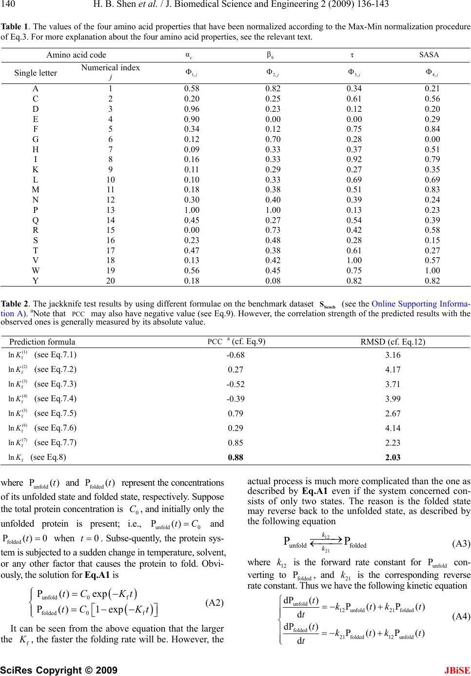 140 H. B. Shen et al. / J. Biomedical Science and Engineering 2 (2009) 136-143 SciRes Copyright © 2009 Table 1. The values of the four amino acid properties that have been normalized according to the Max-Min normalization procedure of Eq.3. For more explanation about the four amino acid properties, see the relevant text. Amino acid code c α S β τ SASA Single letter Numerical index j1, 2, 3, 4, A 1 0.58 0.82 0.34 0.21 C 2 0.20 0.25 0.61 0.56 D 3 0.96 0.23 0.12 0.20 E 4 0.90 0.00 0.00 0.29 F 5 0.34 0.12 0.75 0.84 G 6 0.12 0.70 0.28 0.00 H 7 0.09 0.33 0.37 0.51 I 8 0.16 0.33 0.92 0.79 K 9 0.11 0.29 0.27 0.35 L 10 0.10 0.33 0.69 0.69 M 11 0.18 0.38 0.51 0.83 N 12 0.30 0.40 0.39 0.24 P 13 1.00 1.00 0.13 0.23 Q 14 0.45 0.27 0.54 0.39 R 15 0.00 0.73 0.42 0.58 S 16 0.23 0.48 0.28 0.15 T 17 0.47 0.38 0.61 0.27 V 18 0.13 0.42 1.00 0.57 W 19 0.56 0.45 0.75 1.00 Y 20 0.18 0.08 0.82 0.82 Table 2. The jackknife test results by using different formulae on the benchmark dataset bench (see the Online Supporting Informa- tion A). aNote that PCC may also have negative value (see Eq.9). However, the correlation strength of the predicted results with the observed ones is generally measured by its absolute value. S Prediction formula PCC a (cf. Eq.9) RMSD (cf. Eq.12) (1) f ln (see Eq.7.1) -0.68 3.16 (2) f ln (see Eq.7.2) 0.27 4.17 (3) f ln (see Eq.7.3) -0.52 3.71 (4) f ln (see Eq.7.4) -0.39 3.99 (5) f ln (see Eq.7.5) 0.79 2.67 (6) f ln (see Eq.7.6) 0.29 4.14 (7) f ln (see Eq.7.7) 0.85 2.23 f ln (see Eq.8) 0.88 2.03 where and represent the concentrations of its unfolded state and folded state, respectively. Suppose the total protein concentration is , and initially only the unfolded protein is present; i.e., and when . Subse-quently, the protein sys- tem is subjected to a sudden change in temperature, solvent, or any other factor that causes the protein to fold. Obvi- ously, the solution for Eq.A1 is unfold P(t )0t ) folded P()t 0t 0 C unfold 0 P()tC folded P( JBiSE unfold 0f folded 0f P()exp P() 1exp tC Kt tC Kt (A2) It can be seen from the above equation that the larger the f , the faster the folding rate will be. However, the actual process is much more complicated than the one as described by Eq.A1 even if the system concerned con- sists of only two states. The reason is the folded state may reverse back to the unfolded state, as described by the following equation 12 21 unfold folded P k k P (A3) where is the forward rate constant for con- verting to folded , and 21 is the corresponding reverse rate constant. Thus we have the following kinetic equation 12 kunfold P Pk unfold 12unfold21folded folded 21 folded12 unfold dP( )P() P( d dP( )P() P( d tktk ttktk t ) ) t t (A4) 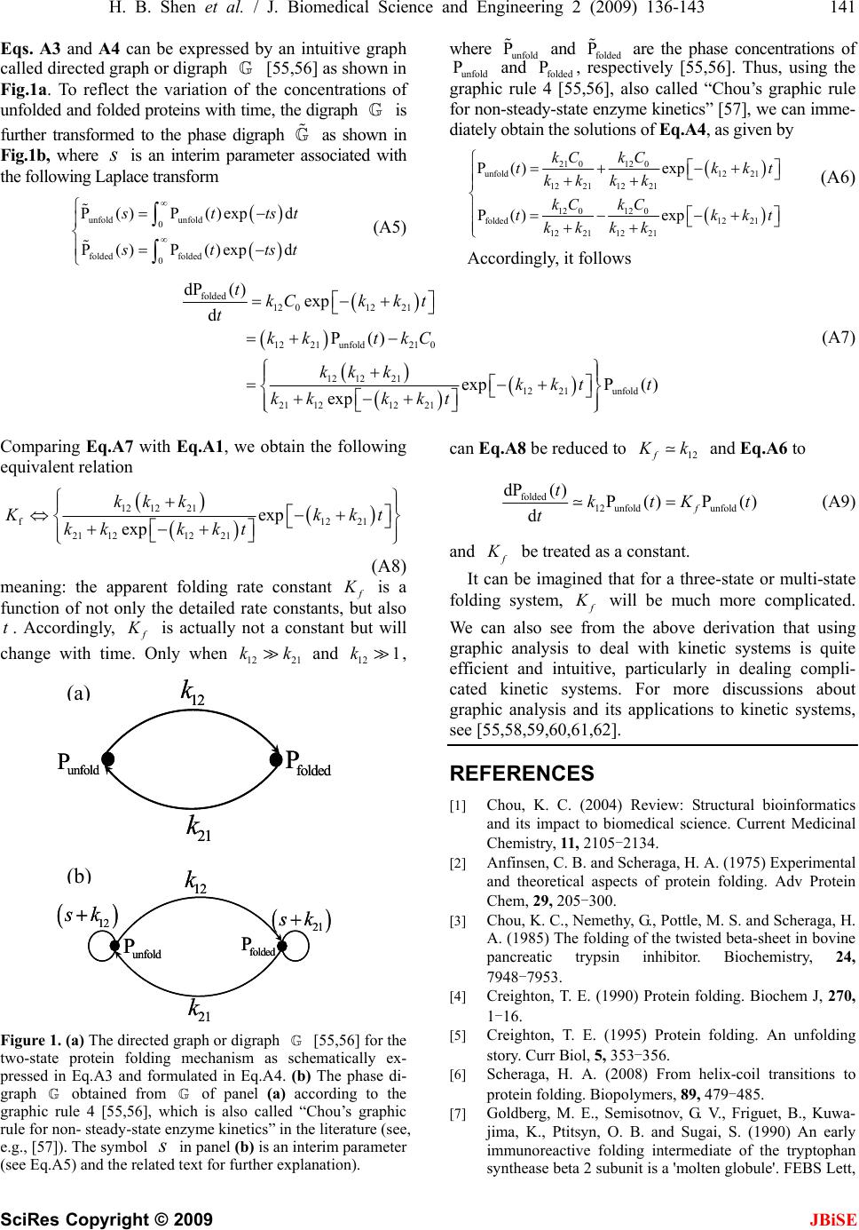 H. B. Shen et al. / J. Biomedical Science and Engineering 2 (2009) 136-143 141 SciRes Copyright © 2009 JBiSE Eqs. A3 and A4 can be expressed by an intuitive graph called directed graph or digraph [55,56] as shown in Fig.1a. To reflect the variation of the concentrations of unfolded and folded proteins with time, the digraph is further transformed to the phase digraph as shown in Fig.1b, where is an interim parameter associated with the following Laplace transform s unfold unfold 0 folded folded 0 P()P()expd P() P()expd tts where unfold and folded are the phase concentrations of and , respectively [55,56]. Thus, using the P P P unfold folded graphic rule 4 [55,56], also called “Chou’s graphic rule for non-steady-state enzyme kinetics” [57], we can imme- diately obtain the solutions of Eq.A4, as given by P 21 012 0 unfold12 21 12 211221 12 012 0 folded12 21 12 2112 21 P() exp P()exp kC kC tk kkkk kC kC tk kkkk kt kt (A6) t tts t (A5) Accordingly, it follows folded 12 01221 1221unfold21 0 12 1221 12 21unfold 21 121221 dP( )exp d P() expP() exp tkCkk t t kk tkC kk kkkt t kk kkt (A7) Comparing Eq.A7 with Eq.A1, we obtain the following equivalent relation 12 1221 f12 21 121221 exp exp kk k 21 kkt kk kkt (A8) meaning: the apparent folding rate constant f is a function of not only the detailed rate constants, but also . Accordingly, tf is actually not a constant but will change with time. Only when and k, 12 21 kk12 1 Figure 1. (a) The directed graph or digraph [55,56] for the two-state protein folding mechanism as schematically ex- pressed in Eq.A3 and formulated in Eq.A4. (b) The phase di- graph obtained from of panel (a) according to the graphic rule 4 [55,56], which is also called “Chou’s graphic rule for non- steady-state enzyme kinetics” in the literature (see, e.g., [57]). The symbol in panel (b) is an interim parameter (see Eq.A5) and the related text for further explanation). s can Eq.A8 be reduced to 12f k and Eq.A6 to folded 12 unfoldunfold dP( )P() P( df tktK t)t (A9) and f be treated as a constant. It can be imagined that for a three-state or multi-state folding system, f will be much more complicated. We can also see from the above derivation that using graphic analysis to deal with kinetic systems is quite efficient and intuitive, particularly in dealing compli- cated kinetic systems. For more discussions about graphic analysis and its applications to kinetic systems, see [55,58,59,60,61,62]. unfold P 12 k 21 k folded P unfold P 12 k 21 k REFERENCES [1] Chou, K. C. (2004) Review: Structural bioinformatics and its impact to biomedical science. Current Medicinal Chemistry, 11, 2105-2134. [2] Anfinsen, C. B. and Scheraga, H. A. (1975) Experimental and theoretical aspects of protein folding. Adv Protein Chem, 29, 205-300. [3] Chou, K. C., Nemethy, G., Pottle, M. S. and Scheraga, H. A. (1985) The folding of the twisted beta-sheet in bovine pancreatic trypsin inhibitor. Biochemistry, 24, 7948-7953. [4] Creighton, T. E. (1990) Protein folding. Biochem J, 270, 1-16. [5] Creighton, T. E. (1995) Protein folding. An unfolding story. Curr Biol, 5, 353-356. [6] Scheraga, H. A. (2008) From helix-coil transitions to protein folding. Biopolymers, 89, 479-485. [7] Goldberg, M. E., Semisotnov, G. V., Friguet, B., Kuwa- jima, K., Ptitsyn, O. B. and Sugai, S. (1990) An early immunoreactive folding intermediate of the tryptophan synthease beta 2 subunit is a 'molten globule'. FEBS Lett, folded P unfold Pfolded P 12 k 21 k 12 k 21 k unfold Pfolded P 12 k 21 k 12 k 21 k 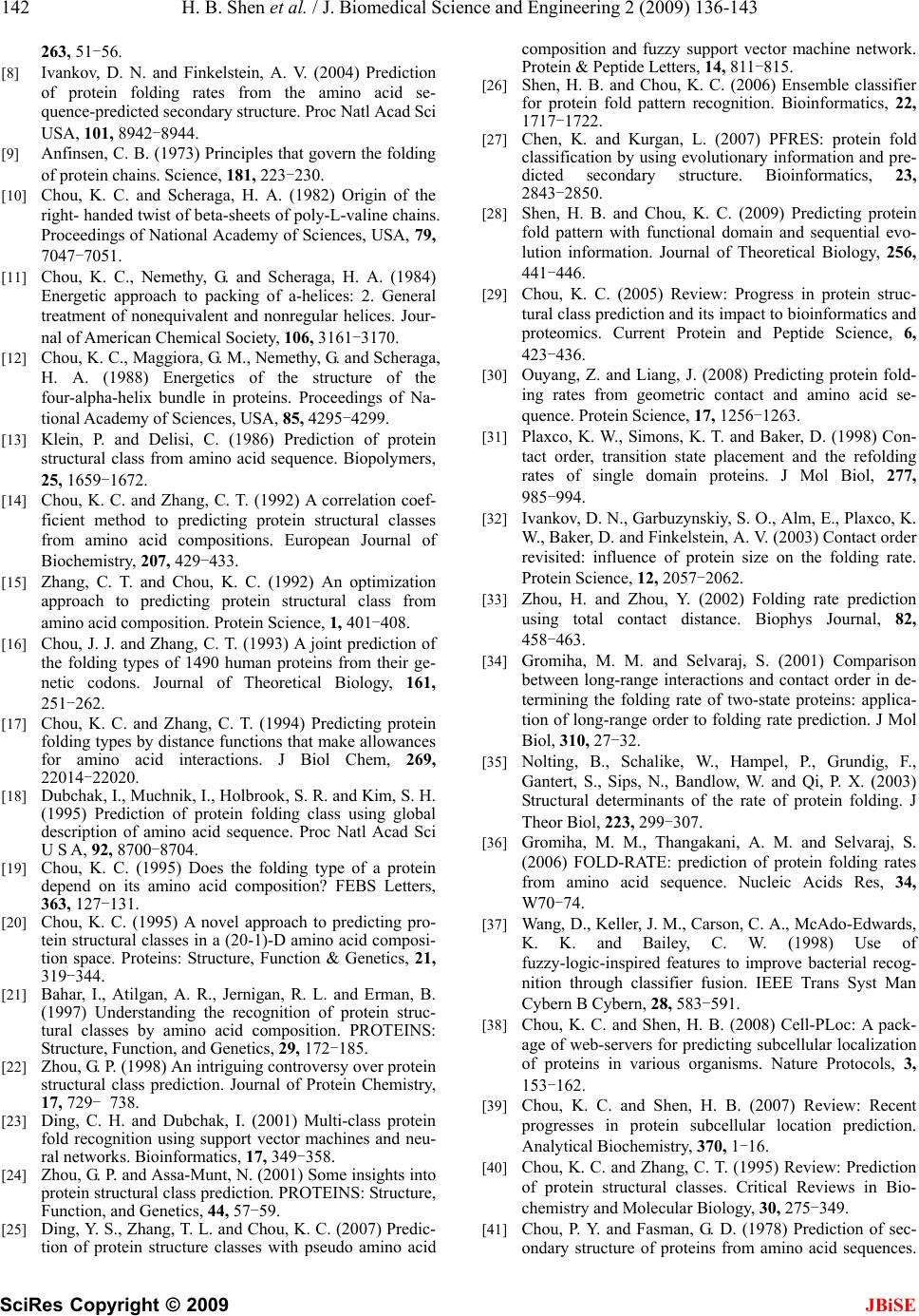 142 H. B. Shen et al. / J. Biomedical Science and Engineering 2 (2009) 136-143 SciRes Copyright © 2009 JBiSE 263, 51-56. [8] Ivankov, D. N. and Finkelstein, A. V. (2004) Prediction of protein folding rates from the amino acid se- quence-predicted secondary structure. Proc Natl Acad Sci USA, 101, 8942-8944. [9] Anfinsen, C. B. (1973) Principles that govern the folding of protein chains. Science, 181, 223-230. [10] Chou, K. C. and Scheraga, H. A. (1982) Origin of the right- handed twist of beta-sheets of poly-L-valine chains. Proceedings of National Academy of Sciences, USA, 79, 7047-7051. [11] Chou, K. C., Nemethy, G. and Scheraga, H. A. (1984) Energetic approach to packing of a-helices: 2. General treatment of nonequivalent and nonregular helices. Jour- nal of American Chemical Society, 106, 3161-3170. [12] Chou, K. C., Maggiora, G. M., Nemethy, G. and Scheraga, H. A. (1988) Energetics of the structure of the four-alpha-helix bundle in proteins. Proceedings of Na- tional Academy of Sciences, USA, 85, 4295-4299. [13] Klein, P. and Delisi, C. (1986) Prediction of protein structural class from amino acid sequence. Biopolymers, 25, 1659-1672. [14] Chou, K. C. and Zhang, C. T. (1992) A correlation coef- ficient method to predicting protein structural classes from amino acid compositions. European Journal of Biochemistry, 207, 429-433. [15] Zhang, C. T. and Chou, K. C. (1992) An optimization approach to predicting protein structural class from amino acid composition. Protein Science, 1, 401-408. [16] Chou, J. J. and Zhang, C. T. (1993) A joint prediction of the folding types of 1490 human proteins from their ge- netic codons. Journal of Theoretical Biology, 161, 251-262. [17] Chou, K. C. and Zhang, C. T. (1994) Predicting protein folding types by distance functions that make allowances for amino acid interactions. J Biol Chem, 269, 22014-22020. [18] Dubchak, I., Muchnik, I., Holbrook, S. R. and Kim, S. H. (1995) Prediction of protein folding class using global description of amino acid sequence. Proc Natl Acad Sci U S A, 92, 8700-8704. [19] Chou, K. C. (1995) Does the folding type of a protein depend on its amino acid composition? FEBS Letters, 363, 127-131. [20] Chou, K. C. (1995) A novel approach to predicting pro- tein structural classes in a (20-1)-D amino acid composi- tion space. Proteins: Structure, Function & Genetics, 21, 319-344. [21] Bahar, I., Atilgan, A. R., Jernigan, R. L. and Erman, B. (1997) Understanding the recognition of protein struc- tural classes by amino acid composition. PROTEINS: Structure, Function, and Genetics, 29, 172-185. [22] Zhou, G. P. (1998) An intriguing controversy over protein structural class prediction. Journal of Protein Chemistry, 17, 729- 738. [23] Ding, C. H. and Dubchak, I. (2001) Multi-class protein fold recognition using support vector machines and neu- ral networks. Bioinformatics, 17, 349-358. [24] Zhou, G. P. and Assa-Munt, N. (2001) Some insights into protein structural class prediction. PROTEINS: Structure, Function, and Genetics, 44, 57-59. [25] Ding, Y. S., Zhang, T. L. and Chou, K. C. (2007) Predic- tion of protein structure classes with pseudo amino acid composition and fuzzy support vector machine network. Protein & Peptide Letters, 14, 811-815. [26] Shen, H. B. and Chou, K. C. (2006) Ensemble classifier for protein fold pattern recognition. Bioinformatics, 22, 1717-1722. [27] Chen, K. and Kurgan, L. (2007) PFRES: protein fold classification by using evolutionary information and pre- dicted secondary structure. Bioinformatics, 23, 2843-2850. [28] Shen, H. B. and Chou, K. C. (2009) Predicting protein fold pattern with functional domain and sequential evo- lution information. Journal of Theoretical Biology, 256, 441-446. [29] Chou, K. C. (2005) Review: Progress in protein struc- tural class prediction and its impact to bioinformatics and proteomics. Current Protein and Peptide Science, 6, 423-436. [30] Ouyang, Z. and Liang, J. (2008) Predicting protein fold- ing rates from geometric contact and amino acid se- quence. Protein Science, 17, 1256-1263. [31] Plaxco, K. W., Simons, K. T. and Baker, D. (1998) Con- tact order, transition state placement and the refolding rates of single domain proteins. J Mol Biol, 277, 985-994. [32] Ivankov, D. N., Garbuzynskiy, S. O., Alm, E., Plaxco, K. W., Baker, D. and Finkelstein, A. V. (2003) Contact order revisited: influence of protein size on the folding rate. Protein Science, 12, 2057-2062. [33] Zhou, H. and Zhou, Y. (2002) Folding rate prediction using total contact distance. Biophys Journal, 82, 458-463. [34] Gromiha, M. M. and Selvaraj, S. (2001) Comparison between long-range interactions and contact order in de- termining the folding rate of two-state proteins: applica- tion of long-range order to folding rate prediction. J Mol Biol, 310, 27-32. [35] Nolting, B., Schalike, W., Hampel, P., Grundig, F., Gantert, S., Sips, N., Bandlow, W. and Qi, P. X. (2003) Structural determinants of the rate of protein folding. J Theor Biol, 223, 299-307. [36] Gromiha, M. M., Thangakani, A. M. and Selvaraj, S. (2006) FOLD-RATE: prediction of protein folding rates from amino acid sequence. Nucleic Acids Res, 34, W70-74. [37] Wang, D., Keller, J. M., Carson, C. A., McAdo-Edwards, K. K. and Bailey, C. W. (1998) Use of fuzzy-logic-inspired features to improve bacterial recog- nition through classifier fusion. IEEE Trans Syst Man Cybern B Cybern, 28, 583-591. [38] Chou, K. C. and Shen, H. B. (2008) Cell-PLoc: A pack- age of web-servers for predicting subcellular localization of proteins in various organisms. Nature Protocols, 3, 153-162. [39] Chou, K. C. and Shen, H. B. (2007) Review: Recent progresses in protein subcellular location prediction. Analytical Biochemistry, 370, 1-16. [40] Chou, K. C. and Zhang, C. T. (1995) Review: Prediction of protein structural classes. Critical Reviews in Bio- chemistry and Molecular Biology, 30, 275-349. [41] Chou, P. Y. and Fasman, G. D. (1978) Prediction of sec- ondary structure of proteins from amino acid sequences.  H. B. Shen et al. / J. Biomedical Science and Engineering 2 (2009) 136-143 143 SciRes Copyright © 2009 JBiSE Advances in Enzymology and Related Subjects in Bio- chemistry, 47, 45-148. [42] Iqbal, M. and Verrall, R. E. (1988) Implications of pro- tein folding. Additivity schemes for volumes and com- pressibilities. J Biol Chem, 263, 4159-4165. [43] Oobatake, M. and Ooi, T. (1993) Hydration and heat stability effects on protein unfolding. Prog Biophys Mol Biol, 59, 237-284. [44] Jones, D. T. (1999) Protein secondary structure predic- tion based on position-specific scoring matrices. J Mol Biol, 292, 195-202. [45] Chou, K. C. (1999) Using pair-coupled amino acid com- position to predict protein secondary structure content. Journal of Protein Chemistry, 18, 473-480. [46] Zhou, X. B., Chen, C., Li, Z. C. and Zou, X. Y. (2007) Using Chou's amphiphilic pseudo-amino acid composi- tion and support vector machine for prediction of enzyme subfamily classes. Journal of Theoretical Biology, 248, 546-551. [47] Ding, Y. S. and Zhang, T. L. (2008) Using Chou's pseudo amino acid composition to predict subcellular localiza- tion of apoptosis proteins: an approach with immune ge- netic algorithm-based ensemble classifier. Pattern Rec- ognition Letters, 29, 1887-1892. [48] Zhang, G. Y., Li, H. C. and Fang, B. S. (2008) Predicting lipase types by improved Chou's pseudo-amino acid composition. Protein & Peptide Letters, 15, 1132-1137. [49] Lin, H. (2008) The modified Mahalanobis discriminant for predicting outer membrane proteins by using Chou's pseudo amino acid composition. Journal of Theoretical Biology, 252, 350-356. [50] Li, F. M. and Li, Q. Z. (2008) Predicting protein subcel- lular location using Chou's pseudo amino acid composi- tion and improved hybrid approach. Protein & Peptide Letters, 15, 612- 616. [51] Zhang, G. Y. and Fang, B. S. (2008) Predicting the co- factors of oxidoreductases based on amino acid composi- tion distribution and Chou's amphiphilic pseudo amino acid composition. Journal of Theoretical Biology, 253, 310-315. [52] Lin, H., Ding, H., Feng-Biao Guo, F. B., Zhang, A. Y. and Huang, J. (2008) Predicting subcellular localization of mycobacterial proteins by using Chou's pseudo amino acid composition. Protein & Peptide Letters, 15, 739-744. [53] Munteanu, C. R., Gonzalez-Diaz, H., Borges, F. and de Magalhaes, A. L. (2008) Natural/random protein classi- fication models based on star network topological indices. Journal of Theoretical Biology, 254, 775-783. [54] Rezaei, M. A., Abdolmaleki, P., Karami, Z., Asadabadi, E. B., Sherafat, M. A., Abrishami-Moghaddam, H., Fadaie, M. and Forouzanfar, M. (2008) Prediction of membrane protein types by means of wavelet analysis and cascaded neural networks. Journal of Theoretical Biology, 254, 817-820. [55] Chou, K. C. (1989) Graphical rules in steady and non-steady enzyme kinetics. J Biol Chem, 264, 12074-12079. [56] Chou, K. C. (1990) Review: Applications of graph theory to enzyme kinetics and protein folding kinetics. Steady and non- steady state systems. Biophysical Chemistry, 35, 1-24. [57] Lin, S. X. and Neet, K. E. (1990) Demonstration of a slow conformational change in liver glucokinase by fluorescence spectroscopy. J Biol Chem, 265, 9670-9675. [58] Chou, K. C. and Liu, W. M. (1981) Graphical rules for non-steady state enzyme kinetics. Journal of Theoretical Biology, 91, 637-654. [59] Zhou, G. P. and Deng, M. H. (1984) An extension of Chou's graphical rules for deriving enzyme kinetic equa- tions to system involving parallel reaction pathways. Biochemical Journal, 222, 169-176. [60] Myers, D. and Palmer, G. (1985) Microcomputer tools for steady-state enzyme kinetics. Bioinformatics (original: Computer Applied Bioscience), 1, 105-110. [61] Kuzmic, P., Ng, K. Y. and Heath, T. D. (1992) Mixtures of tight- binding enzyme inhibitors. Kinetic analysis by a recursive rate equation. Anal Biochem, 200, 68-73. [62] Andraos, J. (2008) Kinetic plasticity and the determina- tion of product ratios for kinetic schemes leading to mul- tiple products without rate laws: new methods based on directed graphs. Canadian Journal of Chemistry, 86, 342-357.
|