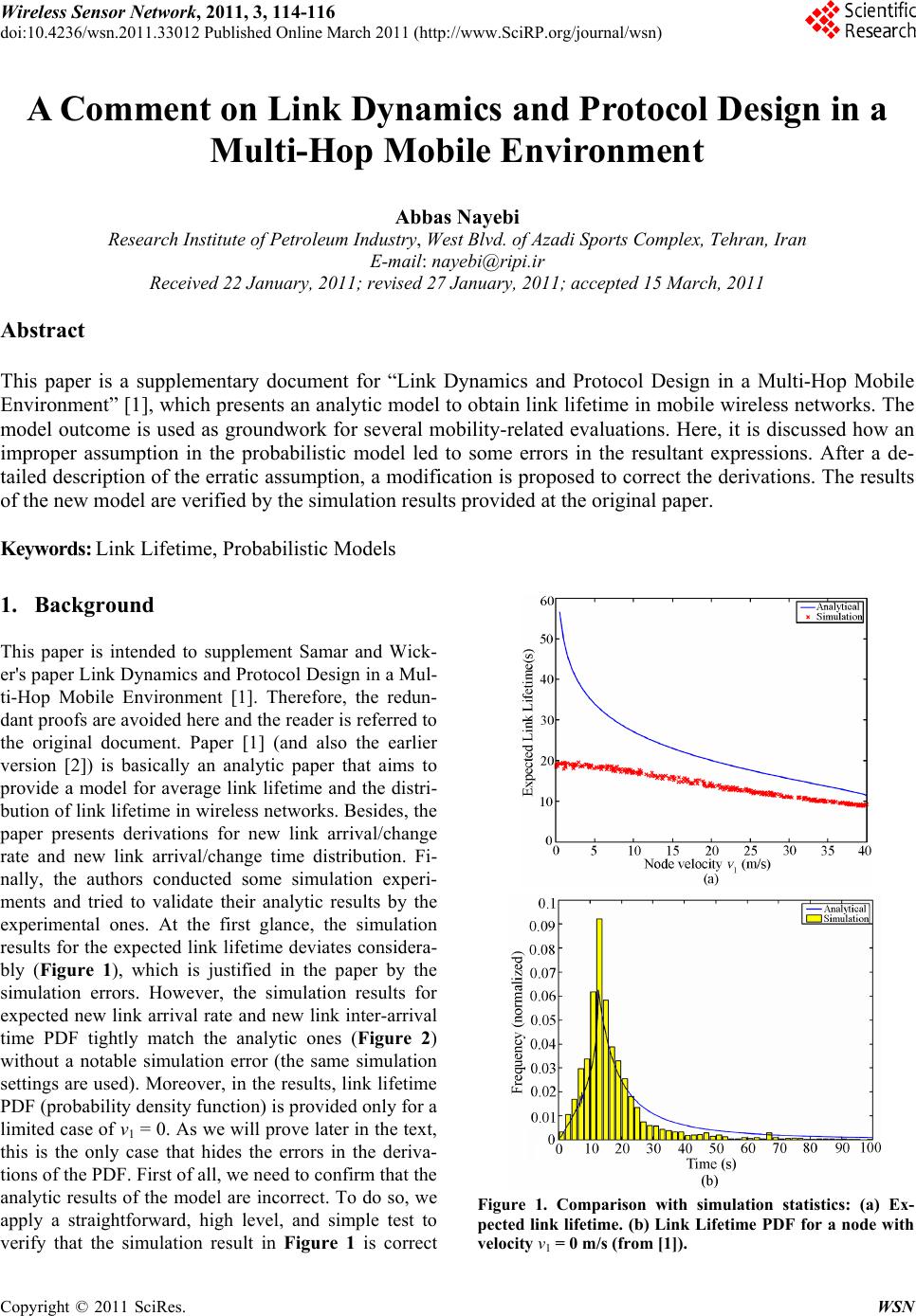Wireless Sensor Network, 2011, 3, 114-116
doi:10.4236/wsn.2011.33012 Published Online March 2011 (http://www.SciRP.org/journal/wsn)
A Comment on Link Dynamics and Protocol Design in a
Multi-Hop Mobile Environment
Abbas Nayebi
Research Institute of Petroleum Industry, West Blvd. of Azadi Sports Complex, Tehran, Iran
Received 22 January, 2011; revised 27 January, 2011; accepted 15 March, 2011
Abstract
This paper is a supplementary document for “Link Dynamics and Protocol Design in a Multi-Hop Mobile
Environment” [1], which presents an analytic model to obtain link lifetime in mobile wireless networks. The
model outcome is used as groundwork for several mobility-related evaluations. Here, it is discussed how an
improper assumption in the probabilistic model led to some errors in the resultant expressions. After a de-
tailed description of the erratic assumption, a modification is proposed to correct the derivations. The results
of the new model are verified by the simulation results provided at the original paper.
Keywords: Link Lifetime, Probabilistic Models
1. Background
This paper is intended to supplement Samar and Wick-
er's paper Link Dynamics and Protocol Design in a Mul-
ti-Hop Mobile Environment [1]. Therefore, the redun-
dant proofs are avoided here and the reader is referred to
the original document. Paper [1] (and also the earlier
version [2]) is basically an analytic paper that aims to
provide a model for average link lifetime and the distri-
bution of link lifetime in wireless networks. Besides, the
paper presents derivations for new link arrival/change
rate and new link arrival/change time distribution. Fi-
nally, the authors conducted some simulation experi-
ments and tried to validate their analytic results by the
experimental ones. At the first glance, the simulation
results for the expected link lifetime deviates considera-
bly (Figure 1), which is justified in the paper by the
simulation errors. However, the simulation results for
expected new link arrival rate and new link inter-arrival
time PDF tightly match the analytic ones (Figure 2)
without a notable simulation error (the same simulation
settings are used). Moreover, in the results, link lifetime
PDF (probability density function) is provided only for a
limited case of v1 = 0. As we will prove later in the text,
this is the only case that hides the errors in the deriva-
tions of the PDF. First of all, we need to confirm that the
analytic results of the model are incorrect. To do so, we
apply a straightforward, high level, and simple test to
verify that the simulation result in Figure 1 is correct
Figure 1. Comparison with simulation statistics: (a) Ex-
pected link lifetime. (b) Link Lifetime PDF for a node with
velocity v1 = 0 m/s (from [1]).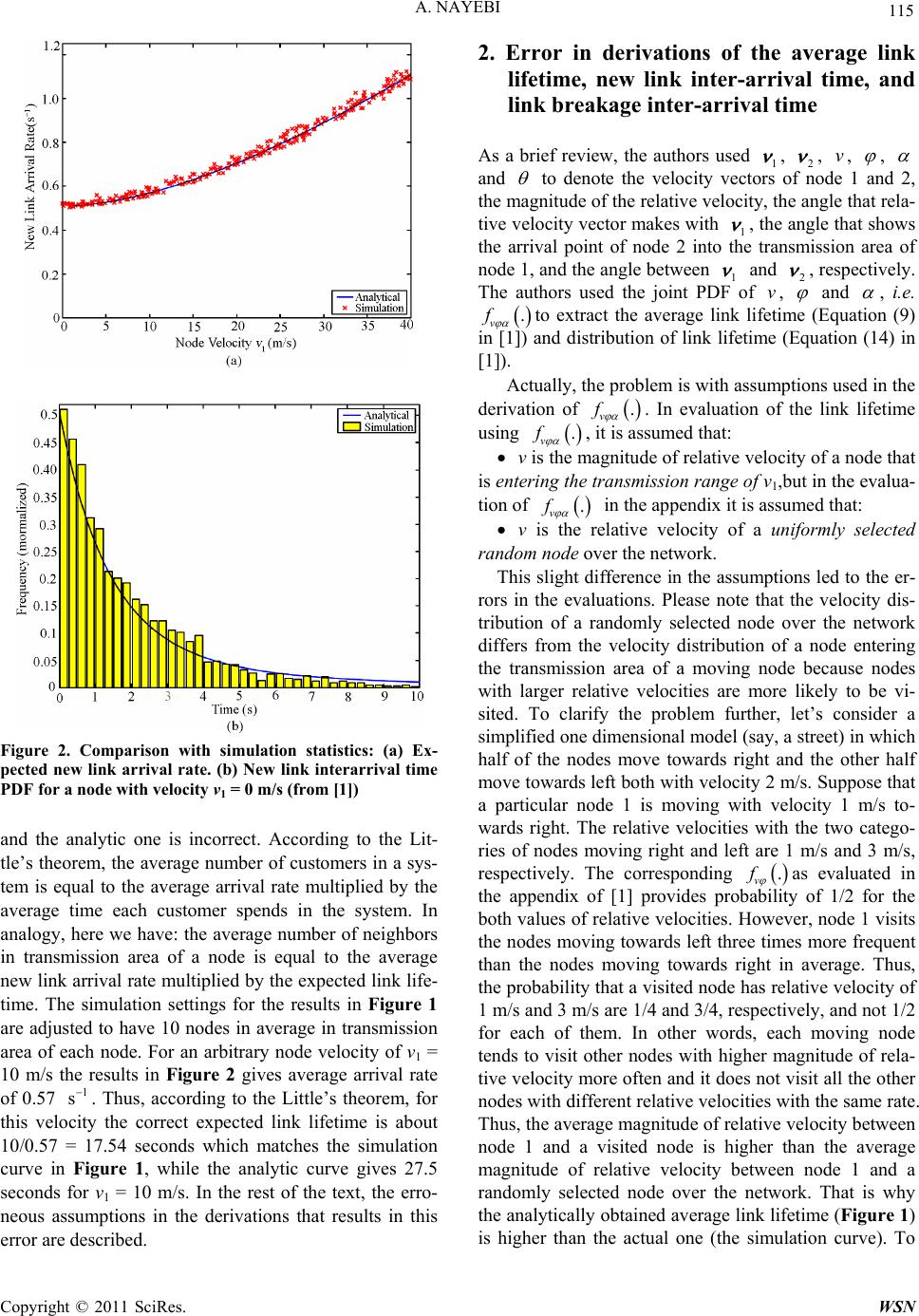

A. NAYEBI
115
Figure 2. Comparison with simulation statistics: (a) Ex-
pected new link arrival rate. (b) New link interarrival time
PDF for a node with velocity v1 = 0 m/s (from [1])
and the analytic one is incorrect. According to the Lit-
tle’s theorem, the average number of customers in a sys-
tem is equal to the average arrival rate multiplied by the
average time each customer spends in the system. In
analogy, here we have: the average number of neighbors
in transmission area of a node is equal to the average
new link arrival rate multiplied by the expected link life-
time. The simulation settings for the results in Figure 1
are adjusted to have 10 nodes in average in transmission
area of each node. For an arbitrary node velocity of v1 =
10 m/s the results in Figure 2 gives average arrival rate
of 0.57 1 s. Thus, according to the Little’s theorem, for
this velocity the correct expected link lifetime is about
10/0.57 = 17.54 seconds which matches the simulation
curve in Figure 1, while the analytic curve gives 27.5
seconds for v1 = 10 m/s. In the rest of the text, the erro-
neous assumptions in the derivations that results in this
error are described.
2. Error in derivations of the average link
lifetime, new link inter-arrival time, and
link breakage inter-arrival time
As a brief review, the authors used 1

, 2

, v,

,

and

to denote the velocity vectors of node 1 and 2,
the magnitude of the relative velocity, the angle that rela-
tive velocity vector makes with 1

, the angle that shows
the arrival point of node 2 into the transmission area of
node 1, and the angle between 1

and 2

, respectively.
The authors used the joint PDF of v,

and

, i.e.


.
v
f

to extract the average link lifetime (Equation (9)
in [1]) and distribution of link lifetime (Equation (14) in
[1]).
Actually, the problem is with assumptions used in the
derivation of


.
v
f

. In evaluation of the link lifetime
using


.
v
f

, it is assumed that:
 v is the magnitude of relative velocity of a node that
is entering the tra nsmission ra nge o f v1,but in the evalua-
tion of


.
v
f

in the appendix it is assumed that:
 v is the relative velocity of a uniformly selected
random node over the network.
This slight difference in the assumptions led to the er-
rors in the evaluations. Please note that the velocity dis-
tribution of a randomly selected node over the network
differs from the velocity distribution of a node entering
the transmission area of a moving node because nodes
with larger relative velocities are more likely to be vi-
sited. To clarify the problem further, let’s consider a
simplified one dimensional model (say, a street) in which
half of the nodes move towards right and the other half
move towards left both with velocity 2 m/s. Suppose that
a particular node 1 is moving with velocity 1 m/s to-
wards right. The relative velocities with the two catego-
ries of nodes moving right and left are 1 m/s and 3 m/s,
respectively. The corresponding


.
v
f

as evaluated in
the appendix of [1] provides probability of 1/2 for the
both values of relative velocities. However, node 1 visits
the nodes moving towards left three times more frequent
than the nodes moving towards right in average. Thus,
the probability that a visited node has relative velocity of
1 m/s and 3 m/s are 1/4 and 3/4, respectively, and not 1/2
for each of them. In other words, each moving node
tends to visit other nodes with higher magnitude of rela-
tive velocity more often and it does not visit all the other
nodes with different relative velocities with the same rate.
Thus, the average magnitude of relative velocity between
node 1 and a visited node is higher than the average
magnitude of relative velocity between node 1 and a
randomly selected node over the network. That is why
the analytically obtained average link lifetime (Figure 1)
is higher than the actual one (the simulation curve). To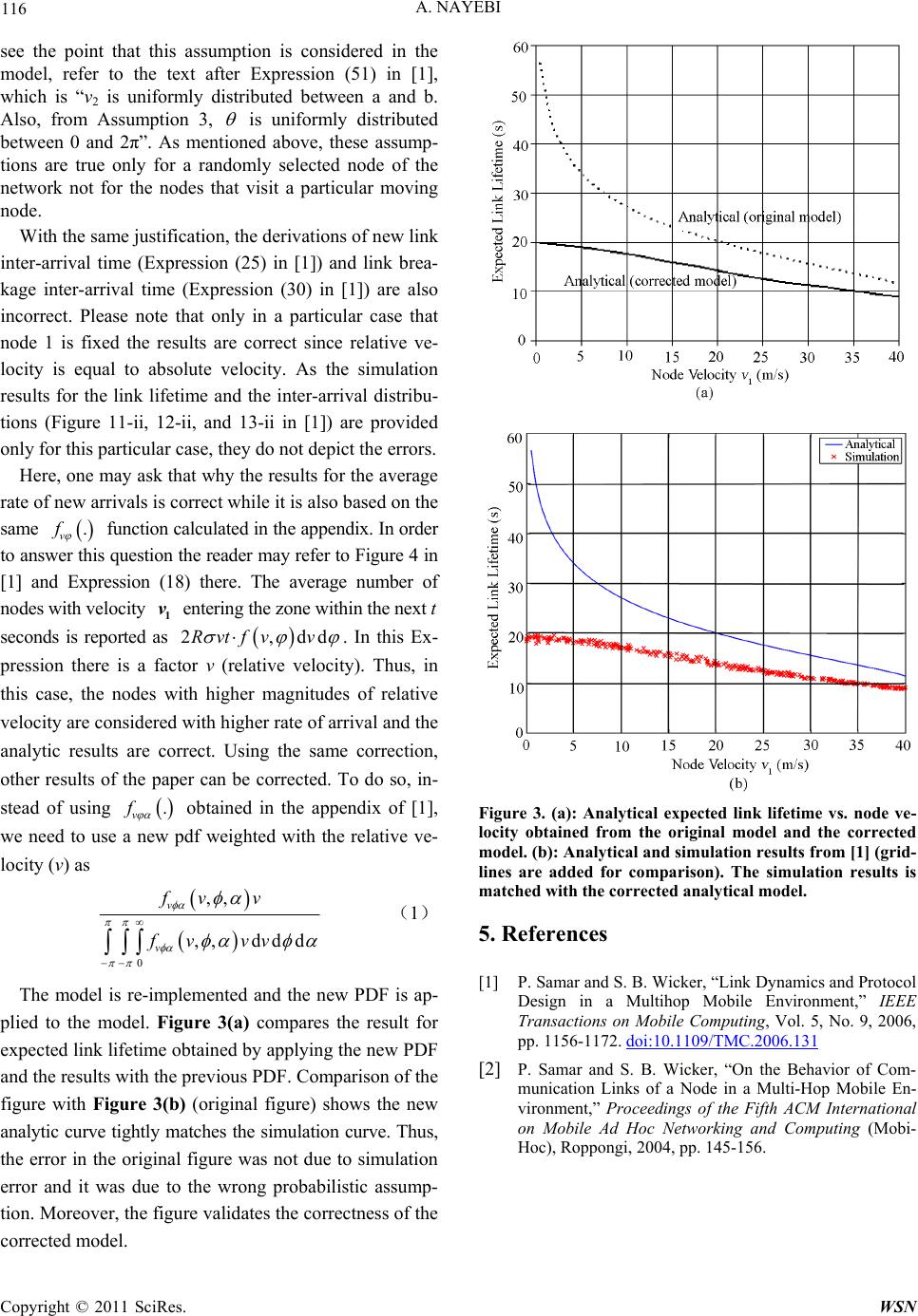

A. NAYEBI
116
see the point that this assumption is considered in the
model, refer to the text after Expression (51) in [1],
which is “v2 is uniformly distributed between a and b.
Also, from Assumption 3,

is uniformly distributed
between 0 and 2π”. As mentioned above, these assump-
tions are true only for a randomly selected node of the
network not for the nodes that visit a particular moving
node.
With the same justification, the derivations of new link
inter-arrival time (Expression (25) in [1]) and link brea-
kage inter-arrival time (Expression (30) in [1]) are also
incorrect. Please note that only in a particular case that
node 1 is fixed the results are correct since relative ve-
locity is equal to absolute velocity. As the simulation
results for the link lifetime and the inter-arrival distribu-
tions (Figure 11-ii, 12-ii, and 13-ii in [1]) are provided
only for this particular case, they do not depict the errors.
Here, one may ask that why the results for the average
rate of new arrivals is correct while it is also based on the
same

.
v
f

function calculated in the appendix. In order
to answer this question the reader may refer to Figure 4 in
[1] and Expression (18) there. The average number of
nodes with velocity 1 v entering the zone within the next t
seconds is reported as

2,ddRvtfv v

 . In this Ex-
pression there is a factor v (relative velocity). Thus, in
this case, the nodes with higher magnitudes of relative
velocity are considered with higher rate of arrival and the
analytic results are correct. Using the same correction,
other results of the paper can be corrected. To do so, in-
stead of using

.
v
f

obtained in the appendix of [1],
we need to use a new pdf weighted with the relative ve-
locity (v) as


0
,,
,, ddd
v
v
fv v
fv vv










（1）
The model is re-implemented and the new PDF is ap-
plied to the model. Figure 3(a) compares the result for
expected link lifetime obtained by applying the new PDF
and the results with the previous PDF. Comparison of the
figure with Figure 3(b) (original figure) shows the new
analytic curve tightly matches the simulation curve. Thus,
the error in the original figure was not due to simulation
error and it was due to the wrong probabilistic assump-
tion. Moreover, the figure validates the correctness of the
corrected model.
Figure 3. (a): Analytical expected link lifetime vs. node ve-
locity obtained from the original model and the corrected
model. (b): Analytical and simulation results from [1] (grid-
lines are added for comparison). The simulation results is
matched with the corrected analytical model.
5. References
[1] P. Samar and S. B. Wicker, “Link Dynamics and Protocol
Design in a Multihop Mobile Environment,” IEEE
Transactions on Mobile Computing, Vol. 5, No. 9, 2006,
pp. 1156-1172. doi:10.1109/TMC.2006.131
[2] P. Samar and S. B. Wicker, “On the Behavior of Com-
munication Links of a Node in a Multi-Hop Mobile En-
vironment,” Proceedings of the Fifth ACM International
on Mobile Ad Hoc Networking and Computing (Mobi-
Hoc), Roppongi, 2004, pp. 145-156.