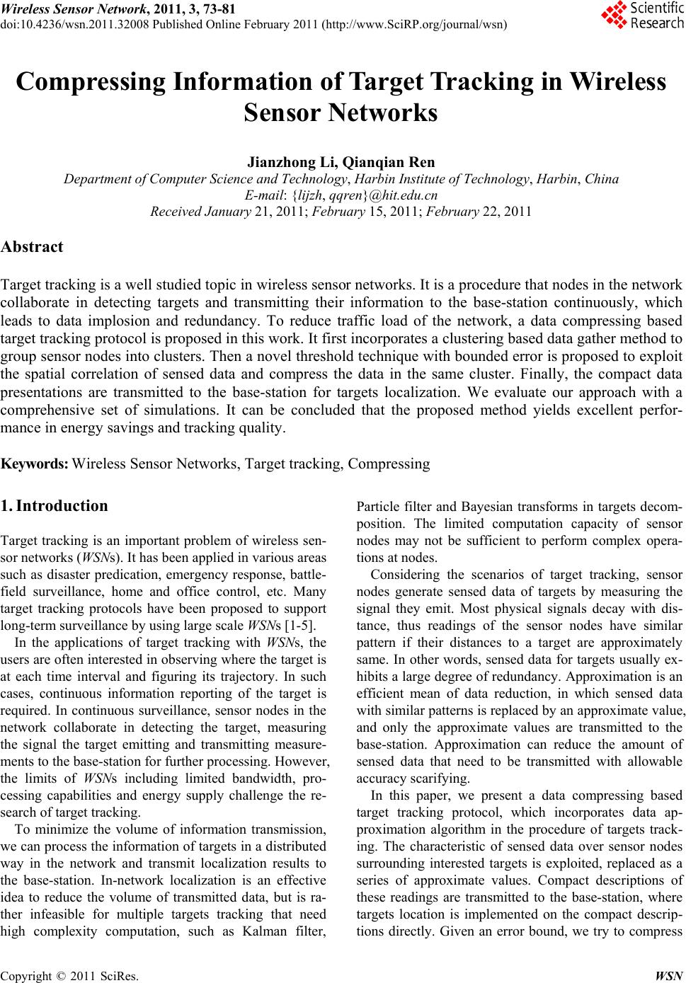Wireless Sensor Network, 2011, 3, 73-81
doi:10.4236/wsn.2011.32008 Published Online February 2011 (http://www.SciRP.org/journal/wsn)
Compressing Information of Target Tracking in Wireless
Sensor Networks
Jianzhong Li, Qianqian Ren
Department of C omput er Science and Techn olo gy, Harbin Institute of Technology, Harbin , China
Received January 21, 2011; February 15, 2011; February 22, 2011
Abstract
Target tracking is a well studied topic in wireless sensor networks. It is a procedure that nodes in the network
collaborate in detecting targets and transmitting their information to the base-station continuously, which
leads to data implosion and redundancy. To reduce traffic load of the network, a data compressing based
target tracking protocol is proposed in this work. It first incorporates a clustering based data gather method to
group sensor nodes into clusters. Then a novel threshold technique with bounded error is proposed to exploit
the spatial correlation of sensed data and compress the data in the same cluster. Finally, the compact data
presentations are transmitted to the base-station for targets localization. We evaluate our approach with a
comprehensive set of simulations. It can be concluded that the proposed method yields excellent perfor-
mance in energy savings and tracking quality.
Keywords: Wireless Sensor Networks, Target tracking, Compressing
1. Introduction
Target tracking is an important problem of wireless sen-
sor networks (WSNs). It has been applied in various areas
such as disaster predication, emergency response, battle-
field surveillance, home and office control, etc. Many
target tracking protocols have been proposed to support
long-term surveillance by using large scale WSNs [1-5].
In the applications of target tracking with WSNs, the
users are often interested in observing where the target is
at each time interval and figuring its trajectory. In such
cases, continuous information reporting of the target is
required. In continuous surveillance, sensor nodes in the
network collaborate in detecting the target, measuring
the signal the target emitting and transmitting measure-
ments to the base-station for further processing. However,
the limits of WSNs including limited bandwidth, pro-
cessing capabilities and energy supply challenge the re-
search of target tracking.
To minimize the volume of information transmission,
we can process the information of targets in a distributed
way in the network and transmit localization results to
the base-station. In-network localization is an effective
idea to reduce the volume of transmitted data, but is ra-
ther infeasible for multiple targets tracking that need
high complexity computation, such as Kalman filter,
Particle filter and Bayesian transforms in targets decom-
position. The limited computation capacity of sensor
nodes may not be sufficient to perform complex opera-
tions at nodes.
Considering the scenarios of target tracking, sensor
nodes generate sensed data of targets by measuring the
signal they emit. Most physical signals decay with dis-
tance, thus readings of the sensor nodes have similar
pattern if their distances to a target are approximately
same. In other words, sensed data for targets usually ex-
hibits a large deg ree of redundancy. App roximation is an
efficient mean of data reduction, in which sensed data
with similar patterns is replaced by an approximate value,
and only the approximate values are transmitted to the
base-station. Approximation can reduce the amount of
sensed data that need to be transmitted with allowable
accuracy scarifying.
In this paper, we present a data compressing based
target tracking protocol, which incorporates data ap-
proximation algorithm in the procedure of targets track-
ing. The characteristic of sensed data over sensor nodes
surrounding interested targets is exploited, replaced as a
series of approximate values. Compact descriptions of
these readings are transmitted to the base-station, where
targets location is implemented on the compact descrip-
tions directly. Given an error bound, we try to compress

J. Z. LI ET AL.
74
readings for the same target maximally by grouping the
original data and approximating them falls within the
error bound around estimated values. The proposed ap-
proach can release the traffic load and reduce energy
consumption for data transmission efficiently. However,
this often comes at the price of loss in tracking quality,
which is equivalent to a lo ss in data precision and locali-
zation accuracy. We analyze the error of tracking results
and discuss the determinations of parameters in the paper.
In addition, the proposed compressing provides a low
overhead, which makes it practical for overh ead sens itive
applications with WSNs.
The contributions of this paper are as follows:
 We introduce a new approximation scheme that
makes full use of correlations among data of mul-
tiple sensor nodes. It exploits the spatial co rrelation
of targets information to implement data reduction.
 We incorporate the idea of data reduction into tar-
get tracking, which shrinks the volume of trans-
mitted data efficiently with guarantee of tracking
quality. It is an efficient solution for prolonged
network lifetime.
 We explore the trade-off between energy savings
and tracking quality. We aim to design a tracking
system in an energy-efficient manner at the price of
allowable accuracy sacrificing.
 We provide an extensive experiments and analysis
of our framework using a simulated sensor network.
Experimental results show that our approach achie-
ves well performance in terms of tracking quality
and energy conservation.
The remainder of this paper is organized as follows.
Related work is shown in Section 2. We give the network
model in Section 3. A data compressing based tracking
protocol is detailed in Section 4. We analyze the perfor-
mance of proposed technique in Section 5. Section 6
presents detailed simulations. Finally, we conclude this
paper in Section 7.
2. Related Work
In recent years, many research works have been provided
in the area of target tracking using WSNs. The important
issues studied mainly include energy efficient tracking
and accurate tracking.
The authors in [6-9] adopt binary sensor model to
track targets. The output of each binary sensor is only
one bit (0 or 1). The binary sensor nodes based tracking
can conserve the energy for data transmissions efficiently.
However, this kind of nodes does not have the capacity
of calculation, and any loss of packets may affect the
tracking accuracy evidently. Some works address the
problem of energy efficiency by reducing the number of
nodes participating in working. In [10], a distributed
tracking algorithm using dynamic conveying tree struc-
ture is presented, which optimizes the problem of target
tracking by building a convoy tree sequence with high
tree coverage and low energy consumption. The work of
[11] proposes an information-driven tracking approach
by deciding the collaboration of sensor nodes consider-
ing the constraints of information and resource consump-
tion.
The authors in [2] propo se a minimal contour-track ing
model to minimize the number of nodes involved in
tracking. It searches for the minimal tracking area based
on the vehicular kinematics to minimize working nodes.
In [12], the problem of tracking mobile nodes is ad-
dressed by measuring the Doppler shifts of the transmit-
ted signal. Moreover, the extended Kalman filter is
adopted to remove the effects of the measurement errors
in sensor networks with uncertainty. The distributed al-
gorithms for in-network tracking and range queries are
proposed in [13], they use differential one-form in the
application of target tracking to search for a given id enti-
fiable target with low time complexity. The proposed
approaches are also flexible to network changes and
node mobility.
The above tracking techniques focus on reducing
transmission amounts or the number of nodes participat-
ing in work.
To further reduce energy consumption in the long-
term surveillance, nodes scheduling is app lied in moving
target tracking systems [4,14,15]. A real-time target
tracking system with WSNs is designed in [3,4], which
adopts an energy management scheme to make sensor
nodes rotate in active and sleep state to conserve energy
of the network. Moreover, some scheduling and wake-up
topics are analyzed. In [14], an optimal node sleep sche-
duling protocol for rare-event detection is proposed. A
deterministically rotating sensory coverage with con-
strains of detection delay is developed. The authors of
[15] study the problem of network deployment and de-
sign an efficient scheduling protocol. It wakes up and
shuts down sensor nodes with certain spatial and tem-
poral preciseness.
These existing techniques mainly focus on the tracking
and searching of a single target, it is not adaptable to
multiple targets tracking. The authors of [2] study fault
tolerant tracking. The Gaussian mixture model is intro-
duced to capture the characteristics of the target signal.
In addition, a temporally adaptive variant of the approach
is proposed to track dynamic multiple targets under
changing environments, with noisy considering. While
the focus of [2] is accurately tracking moving targets
with noise considering. In this paper, we propose a real
time target tracking protocol with energy savings and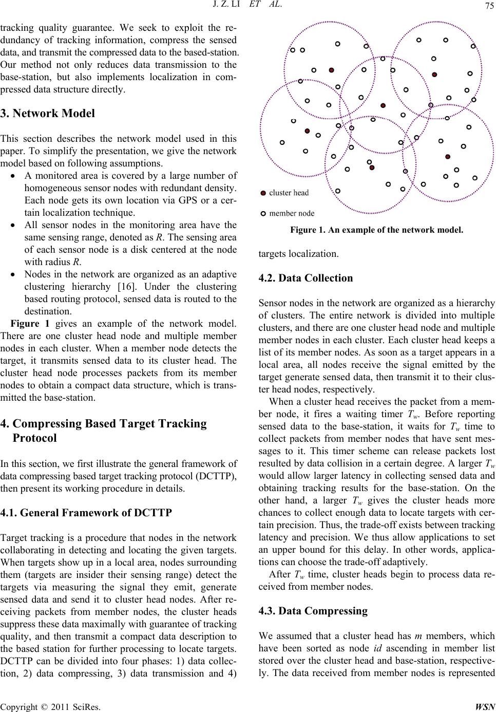

J. Z. LI ET AL.
75
tracking quality guarantee. We seek to exploit the re-
dundancy of tracking information, compress the sensed
data, and transmit the compressed data to the based-station.
Our method not only reduces data transmission to the
base-station, but also implements localization in com-
pressed data structure directly.
3. Network Model
This section describes the network model used in this
paper. To simplify the presentation, we give the network
model based on following assumptions.
 A monitored area is covered by a large number of
homogeneous sensor nodes with redundant density.
Each node gets its own location via GPS or a cer-
tain localization technique.
 All sensor nodes in the monitoring area have the
same sensing range, denoted as R. The sensing are a
of each sensor node is a disk centered at the node
with radius R.
 Nodes in the network are organized as an adaptive
clustering hierarchy [16]. Under the clustering
based routing protocol, sensed data is routed to the
destination.
Figure 1 gives an example of the network model.
There are one cluster head node and multiple member
nodes in each cluster. When a member node detects the
target, it transmits sensed data to its cluster head. The
cluster head node processes packets from its member
nodes to obtain a compact data structure, which is trans-
mitted the base-station.
4. Compressing Based Target Tracking
Protocol
In this section , we first illustra te the general fra mework of
data compressing based target tracking protocol (DCTTP),
then present its working pro c edure in details.
4.1. General Framework of DCTTP
Target tracking is a procedure that nodes in the network
collaborating in detecting and locating the given targets.
When targets show up in a local area, nodes surrounding
them (targets are insider their sensing range) detect the
targets via measuring the signal they emit, generate
sensed data and send it to cluster head nodes. After re-
ceiving packets from member nodes, the cluster heads
suppress these data maximally with guarantee of tracking
quality, and then transmit a compact data description to
the based station for further processing to locate targets.
DCTTP can be divided into four phases: 1) data collec-
tion, 2) data compressing, 3) data transmission and 4)
Figure 1. An example of the network model.
targets localization.
4.2. Data Collection
Sensor nodes in the network are organized as a hierarchy
of clusters. The entire network is divided into multiple
clusters, and there are one cluster head node and multiple
member nodes in each cluster. Each cluster head keeps a
list of its member nodes. As soon as a targ et appears in a
local area, all nodes receive the signal emitted by the
target generate sensed data, then transmit it to their clus-
ter head nodes, respectively.
When a cluster head receives the packet from a mem-
ber node, it fires a waiting timer Tw. Before reporting
sensed data to the base-station, it waits for Tw time to
collect packets from member nodes that have sent mes-
sages to it. This timer scheme can release packets lost
resulted by data collision in a certain degree. A larg er Tw
would allow larger latency in collecting sensed data and
obtaining tracking results for the base-station. On the
other hand, a larger Tw gives the cluster heads more
chances to collect enough data to locate targets with cer-
tain precision. Thus, the trade-off exists between tracking
latency and precision. We thus allow applications to set
an upper bound for this delay. In other words, applica-
tions can choose the trade-off adaptively.
After Tw time, cluster heads begin to process data re-
ceived from mem ber no des.
4.3. Data Compressing
We assumed that a cluster head has m members, which
have been sorted as node id ascending in member list
stored over the cluster head and base-station, respective-
ly. The data received from member nodes is represented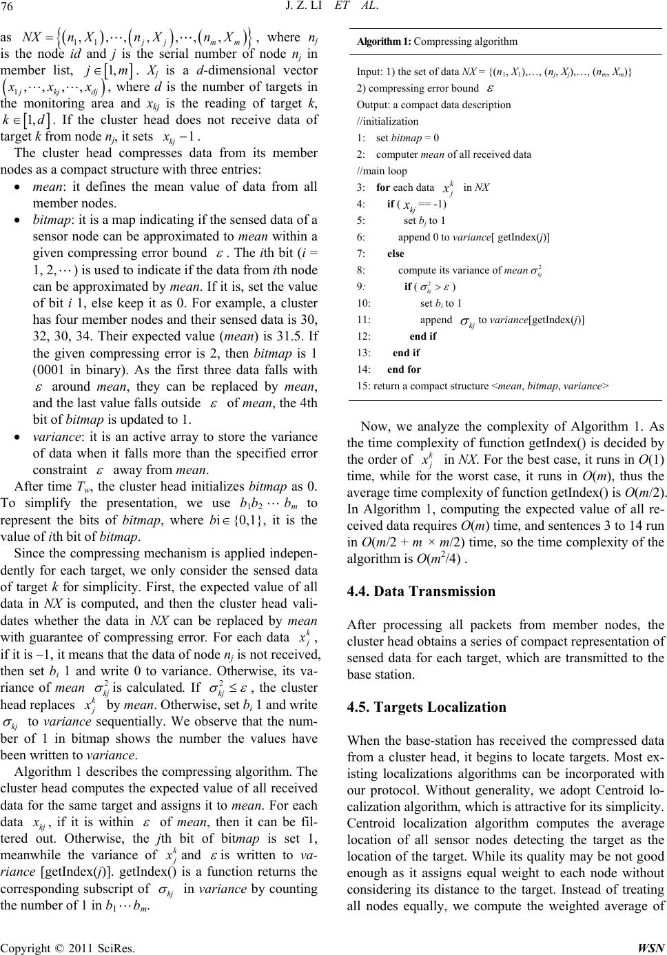

J. Z. LI ET AL.
76
as
 


11
,,,,,,,
jj mm
NXn XnXnX , where nj
is the node id and j is the serial number of node nj in
member list,


1,jm. Xj is a d-dimensional vector

1,,,,
j
kj dj
x
xx , where d is the number of targets in
the monitoring area and xkj is the reading of target k,


1,kd. If the cluster head does not receive data of
target k from node nj, it sets 1
kj
x.
The cluster head compresses data from its member
nodes as a compact structure with three entries:
 mean: it defines the mean value of data from all
member nodes.
 bitmap: it is a map indicating if the sensed data of a
sensor node can be approximated to mean within a
given compressing error bound

. The ith bit (i =
1, 2,) is used to indicate if the data from ith node
can be approximated by mean. If it is, set the value
of bit i 1, else keep it as 0. For example, a cluster
has four member nodes and their sensed data is 30,
32, 30, 34. Their expected value (mean) is 31.5. If
the given compressing error is 2, then bitmap is 1
(0001 in binary). As the first three data falls with

around mean, they can be replaced by mean,
and the last value falls outside

of mean, the 4th
bit of bitmap is updated to 1.
 variance: it is an active array to store the variance
of data when it falls more than the specified error
constraint

away from mean.
After time Tw, the cluster head initializes bitmap as 0.
To simplify the presentation, we use b1b2bm to
represent the bits of bitmap, where bi{0,1}, it is the
value of ith bit of bitmap.
Since the compressing mechanism is applied indepen-
dently for each target, we only consider the sensed data
of target k for simplicity. First, the expected value of all
data in NX is computed, and then the cluster head vali-
dates whether the data in NX can be replaced by mean
with guarantee of compressing error. For each data k
j
x
,
if it is –1, it means that the data of node nj is not received,
then set bi 1 and write 0 to variance. Otherwise, its va-
riance of mean 2
kj

is calculated. If 2
kj

 , the cluster
head replaces k
j
x
by mean. Otherwise, set bi 1 and write
kj

to variance sequentially. We observe that the num-
ber of 1 in bitmap shows the number the values have
been written to variance.
Algorithm 1 describes the compressing algorithm. The
cluster head computes the expected value of all received
data for the same target and assigns it to mean. For each
data kj
x
, if it is within

of mean, then it can be fil-
tered out. Otherwise, the jth bit of bitmap is set 1,
meanwhile the variance of k
j
x
and

is written to va-
riance [getIndex (j)]. getIndex() is a function returns the
corresponding subscript of kj

in variance by counting
the number of 1 in b1bm.
Algorithm 1: Compressing algorithm
Input: 1) the set of data NX = {(n1, X1),…, (nj, Xj),…, (nm, Xm)}
2) compressing error bound

Output: a compact data description
//initialization
1: set bitmap = 0
2: computer mea n of all received data
//main loop
3: for each data k
j
x
in NX
4: if (kj
x
== -1)
5: set bj to 1
6: append 0 to variance[ getInd e x(j)]
7: else
8: compute its variance of mean 2
kj

9: if (2
kj

 )
10: set bi to 1
11: append kj

to variance[getIndex(j)]
12: end if
13: end if
14: end for
15: return a compact structure <mean, bitmap, variance>
Now, we analyze the complexity of Algorithm 1. As
the time complexity of function getIndex() is decided by
the order of k
j
x
in NX. For the best case, it runs in O(1)
time, while for the worst case, it runs in O(m), thus the
average time complexity of function getIndex() is O(m/2).
In Algorithm 1, computing the expected value of all re-
ceived data requires O(m) time, and sentences 3 to 14 run
in O(m/2 + m × m/2) time, so the time complexity of the
algorithm is O(m2/4) .
4.4. Data Transmission
After processing all packets from member nodes, the
cluster head obtains a series of compact representation of
sensed data for each target, which are transmitted to the
base station.
4.5. Targets Localization
When the base-station has received the compressed data
from a cluster head, it begins to locate targets. Most ex-
isting localizations algorithms can be incorporated with
our protocol. Without generality, we adopt Centroid lo-
calization algorithm, which is attractive for its simplicity.
Centroid localization algorithm computes the average
location of all sensor nodes detecting the target as the
location of the target. While its quality may be not good
enough as it assigns equal weight to each node without
considering its distance to the target. Instead of treating
all nodes equally, we compute the weighted average of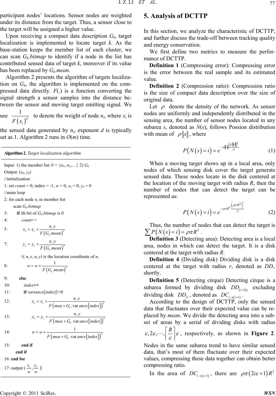

J. Z. LI ET AL.
77
participant nodes’ locations. Sensor nodes are weighted
under its distance from the target. Thus, a sensor close to
the target will be assigned a higher value.
Upon receiving a compact data description Gk, target
localization is implemented to locate target k. As the
base-station keeps the member list of each cluster, we
can scan Gk.bitmap to identify if a node in the list has
contributed sensed data of target k, moreover if its value
has been replaced by Gk.mean.
Algorithm 2 presents the algorithm of targets localiza-
tion on Gk, the algorithm is implemented on the com-
pressed data directly. F(.) is a function converting the
signal strength a sensor samples into the distance be-
tween the sensor and moving target emitting signal. We
use

1
d
i
F
x to denote the weight of node ni, where xi is
the sensed data generated by ni, exponent d is typically
set as 1. Algorithm 2 runs in O(m) time.
Algorithm 2. Target localization algor ithm
Input: 1) the member list N = {n1, n2,…} 2) Gk
Output: (xk, yk)
//initialization
1: set count = 0, index = -1, w = 0, xk = 0, yk = 0
//main loop
2: for each node nj in member list
scan Gk.bitmap
3: if ith bit of Gk.bitmap is 0
4: count++
5:

.
.
id
kk
k
nx
xx
F
Gmean

7:

.
.
id
kk
k
ny
yy
F
Gmean

//( ni.x, ni.y) is the location coordinate of ni
8:

1
.d
k
ww
F
Gmean

9: else
10: index++
11: if variance[index]!=0
12:
 
.
.var
id
kk
k
nx
xxFmeaGance index  
13:


.
.var
id
kk
k
ny
yy
F
meaGance index
 
14:
 
1
.vard
k
ww
F
meaGance index
 
15: end if
end if
16: end for
17: output (,
kk
x
y
ww
)
5. Analysis of DCTTP
In this section, we analyze the characteristic of DCTTP,
and further discuss the trade-off between tracking quality
and energy conservation.
We first define two metrics to measure the perfor-
mance of DCTTP.
Definition 1 (Compressing error): Compressing error
is the error between the real sample and its estimated
value.
Definition 2 (Compression ratio): Compression ratio
is the size of compact data description over the size of
original data.
Let

denote the density of the network. As sensor
nodes are uniformly and independently distributed in the
sensing area, the number of sensor nodes located in any
subarea s, denoted as N(s), follows Possion distribution
with mean of
s

, where
 

!
i
s
si
PNsi e

 
 (1)
When a moving target shows up in a local area, only
nodes of which sensing disk cover the target generate
sensed data. These nodes locate in the disk centered at
the location of the moving target with radius R, then the
number of nodes that can detect the target can be
represented as:
 

2
2!
i
R
Ri
PNsi e

 
 (2)
Thus, the number of nodes that can detect the target is




2
PNsiR  

.
Definition 3 (Detecting area): Detecting area is a local
area, nodes in which can detect the target. It is a disk
centered at the target with radius R.
Definition 4 (Dividing disk) Dividing disk is a disk
centered at the target with radius r, denoted as DDr.
shortly.
Definition 5 (Detecting cirque) Detecting cirque is a
subarea formed by dividing disk

1i
DD

 excluding
dividing disk i DD

, denoted as

1ii
DC .
According to the design of DCTTP, only the sensed
data that fluctuates over their expected value can be re-
placed by mean. We divide the detecting area into a sub-
set of areas by a serial of dividing disks with radius
,2 ,,R









, respectively, as shown in Figure 2.
Nodes in the same subarea trend to have similar sensed
data, that’s most of them fluctuate over their expected
values, compressing these data together can obtain better
compressing ratio.
In the area of

1ii
DC  , there are


2
21iR   

J. Z. LI ET AL.
78
Figure 2. The figure of the sensing area division.
member nodes. Assume that a units are needed to
represent the sensed data and node id, thus, a cluster
head node need transmit

2
221aiR    units data to
report the readings of one target. While with DCTTP, the
cluster head transmits a compact data description of



22
21 121aiRpiRa     
units, where
p is the percentage of the filtered data and
 
2
121piR    is the number of values written to
variance. a units are used to represent mean and

2
21iR    units are used to represent bitmap, re-
spectively.
The compression ratio of data in

1ii
DC  , denoted
as
 1ii
CR can be defined as:



22
12
21 121
221
ii
aiRpiRa
CR aiR
  
 

 

(3)
Setting a = 64, then we have:


12
11 16
64 21
ii
p
CR iR
 


  (4)
Thus, the compression ratio of data in the whole de-
tecting area is:


2
1
2
11 16
64 21
16ln
33 32
64 1
R
whole i
p
CR iR
R
pR
R

 

 













 

 


(5)
In formula (5), parameters R and p are fixed wh en the
network is being deployed. It is clearly that

and p are
two key factors decide the compressing ratio, further
energy conservation of the network.
In theory, sensed data of nodes in the same detecting
cirque can be replaced by their expected value with va-
riances less than

However, measurement errors and
data noisy make var iances of pa rts data be yond

, these
data has to be stored into the item variance of the com-
pact structures.
As the measurement error and data noisy at a certain
node usually follow Gaussian distribution [17]. As p is
decided by the distribution of data and

, thus com-
pressing ratio is in inverse proportion to the given com-
pressing error bound

. That’s energy conservation is at
the cost of data quality sacrificing. We can choose ap-
propriate compressing error according to the moving
mode of targets and experiences to obtain optimal per-
formance of the system.
6. Experiments and Evaluation
In this section, we report our simulation results under
two scenarios: with data noisy and without noisy. In each
case, we report the performance of tracking quality and
energy conservation and our analysis.
In the simulations, sensors nodes are deployed in a re-
gion of 1000 × 1000 unit field. The locations of nodes
are known. All sensor nodes have the same sensing ra-
dius. Three electronic cars are simulated as the targets,
which move along any velocity. For the case with noisy,
we set the mean and variance of Gaussian noise at each
sensor node to 1.
We first define two metrics to measure the perfor-
mance of DCTTP in terms of tracking quality and energy
conservation, that’s tracking error and energy savings
ratio.
Tracking error: It is the average distance between the
real trace of the moving target and its estimated trace.
Energy savings ratio: It is defined as the ratio of
energy savings of DCTTP over the normal tracking sys-
tem without energy conservation mechanisms.
In each scenario, we explore the impact of some key
system configurations on the system performance, such
as network density, sensing range and compressing error.
6.1. Tracking Error
Figure 3 shows the results of tracking error for varying
network density. Fixing sensing range and compressing
error, the numb er of sensor nodes is ranging from 100 to
1000, and the corresponding density varies from 104 to
103. As the increasing of network density, tracking error
decreases obviously. This is because when the network
density is higher, there are more sensor nodes participat-
ing in locating the targets, which generates more sensed
data to be involved in locating multiple targets. The in-
fluence of network density on data with noisy consider-
ing is more serious. As more sensed data helps to fix the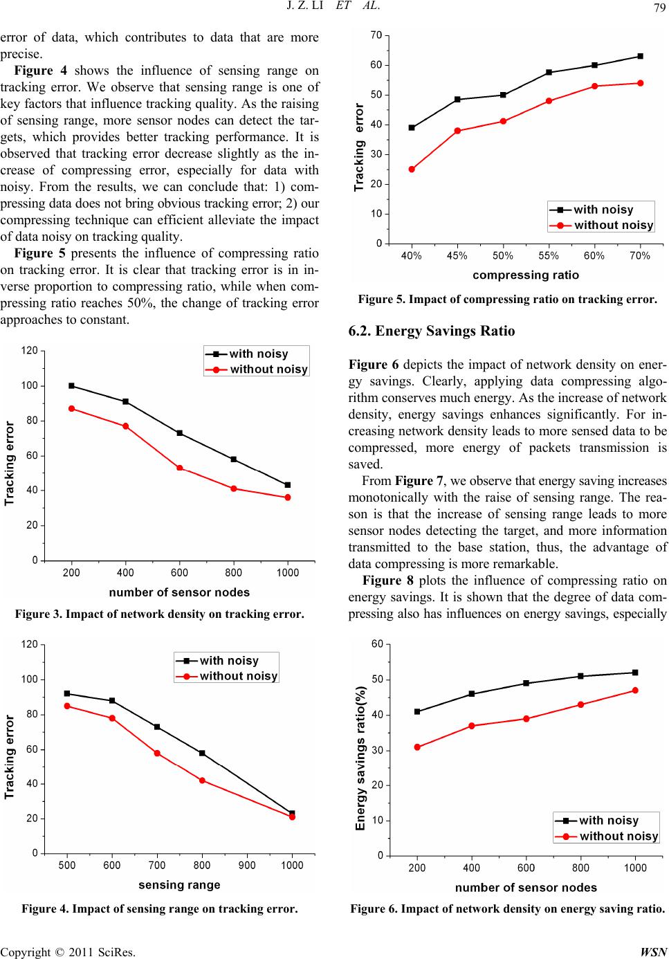

J. Z. LI ET AL.
79
error of data, which contributes to data that are more
precise.
Figure 4 shows the influence of sensing range on
tracking error. We observe that sensing range is one of
key factors that influence tracking quality. As the raising
of sensing range, more sensor nodes can detect the tar-
gets, which provides better tracking performance. It is
observed that tracking error decrease slightly as the in-
crease of compressing error, especially for data with
noisy. From the results, we can conclude that: 1) com-
pressing data does not bring obvious tracking error; 2) our
compressing technique can efficient alleviate the impact
of data noisy on tracking quality.
Figure 5 presents the influence of compressing ratio
on tracking error. It is clear that tracking error is in in-
verse proportion to compressing ratio, while when com-
pressing ratio reaches 50%, the change of tracking error
approaches to constant.
Figure 3. Impact of network density on tracking error.
Figure 4. Impact of sensing range on tracking error.
Figure 5. Impact of compressing ratio on tracking error.
6.2. Energy Savings Ratio
Figure 6 depicts the impact of network density on ener-
gy savings. Clearly, applying data compressing algo-
rithm conserves much energy. As the increase of network
density, energy savings enhances significantly. For in-
creasing network density leads to more sensed data to be
compressed, more energy of packets transmission is
saved.
From Figure 7, we observe that energy saving increases
monotonically with the raise of sensing range. The rea-
son is that the increase of sensing range leads to more
sensor nodes detecting the target, and more information
transmitted to the base station, thus, the advantage of
data compressing is more remarkable.
Figure 8 plots the influence of compressing ratio on
energy savings. It is shown that the degree of data com-
pressing also has influences on energy savings, especially
Figure 6. Impact of network density on energ y s a v i n g rati o .

J. Z. LI ET AL.
80
Figure 7. Impact of sensing range on energy savings ratio.
Figure 8. Impact of compressing ratio on energy savings
ratio.
for data with noisy.
7. Conclusions
In this paper, we concentrate on energy efficient tracking,
dedicated to conserve the whole network energy, as well
as maintain high tracking quality. We have proposed a
data compressing scheme to reduce information trans-
mission of targets. In addition, we incorporate the pro-
posed data compressing technique with tracking protocol
and optimize it to obtain trade-off between energy con-
servation and tracking quality.
We implement a set of simulations to validate our ap-
proach. The results demonstrate the effectiveness of
proposed protocol and illustrate influences of several
parameters on the system. As our future work, we will
implement our tracking algorithm on real sensor nodes.
8. Acknowledgements
This work is partially supported by the NSFC-RGC of
China under Grant No.60831160525, the Key Program
of the National Natural Science Foundation of China
under Gran t No. 61033015, th e National Natural Science
Foundation of China under Grant No. 60933001, the
National Natural Science Foundation of China under
Grant No. 60703012, the Natural Science Foundation of
Heilongjiang Province of China under Grant No. F201038
and the Science and Technology Innovation Research
Project of Harbin for Young Scholar under Grant No.
2009RFQX080.
9. References
[1] Q. Ren, J. Li and H. Gao, “Tpss: A Two-Phase Sleep
Scheduling Protocol for Object Tracking in Sensor Net-
works,” Proceedings of 6th IEEE International Confe-
rence on Mobile Ad-hoc and Sensor Systems, Macao,
2009, pp. 458-465.
[2] Z. Zhong, T. Zhu, D. Wang and T. He, “Tracking with
Unreliable Node Sequences,” INFOCOM, Rio de Janeiro,
19-25 April 2009, pp.1215-1223 .
[3] J. Jeong, T. Hwang, T. He and D. Du, “MCTA: Target
Tracking Algorithm Based on Minimal Contour in Wire-
less Sensor Networks,” Proceedings of 26th Conference
on Computer Communications, Anchorage, 6-12 May
2007, pp. 2371-2375.
[4] T. He, P. A. Vicaire, T. Yan, L. Luo, L. Gu, G. Zhou, R.
Stoleru, Q. Cao, J. A. Stankovic and T. Abdelzaher,
“Achieving Real-Time Target Tracking Using Wireless
Sensor Networks,” ACM Transaction on Embedded
Computing System, 2007.
[5] T. He, P. Vicaire, T. Yan, Q. Cao, G. Zhou, L. Gu, L.
Luo, R. Stoleru, J. A. Stankovic and T. Abdelzaher,
“Achieving Long-Term Surveillance in VigilNet,” Pro-
ceedings of 25th Conference on Computer Communica-
tions, Barcelona, April 2006, pp. 1-12.
[6] N. Shrivastava, R. Mudumbai, U. Madhow and S. Suri,
“Target Tracking with Binary Proximity Sensors: Fun-
damental Limits, Minimal Description, and Algorith,”
ACM Sensys, November 2006.
[7] W. Kim, K. Mechitov, J.-Y. Choi and S. K. Ham, “On
Tracking Objects with Binary Proximity Sensors,” Pro-
ceedings of 4th International Conference on Information
Processing in Sensor Networks, A pr il 2005.
[8] J. Singh, U. Madhow, R. Kumar, S. Suri and R. Cagley,
“Tracking Multiple Targets Using Binary Proximity
Sensors,” Proceedings of 6th International Conference on
Information Processing in Sensor Networks, April 2007.
doi:10.1145/1236360.1236427
[9] Z. J. Wang, E. Bulut, B. K. Szymansky, “Distributed
Energy-Efficient Target Tracking with Binary Sensor
Networks,” ACM Transactions on Sensor Networks, Vol.
6, No. 4, July 2010. doi:10.1145/1777406.1777411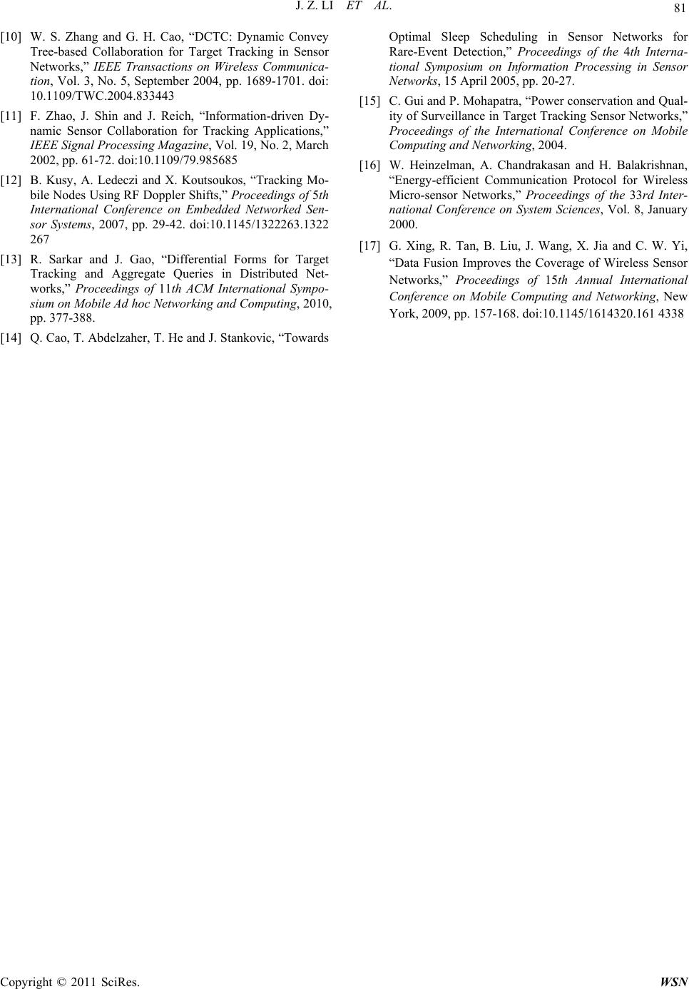

J. Z. LI ET AL.
81
[10] W. S. Zhang and G. H. Cao, “DCTC: Dynamic Convey
Tree-based Collaboration for Target Tracking in Sensor
Networks,” IEEE Transactions on Wireless Communica-
tion, Vol. 3, No. 5, September 2004, pp. 1689-1701. doi:
10.1109/TWC.2004.833443
[11] F. Zhao, J. Shin and J. Reich, “Information-driven Dy-
namic Sensor Collaboration for Tracking Applications,”
IEEE Signal Processing Magazine, Vol. 19, No. 2, March
2002, pp. 61-72. doi:10.1109/79.985685
[12] B. Kusy, A. Ledeczi and X. Koutsoukos, “Tracking Mo-
bile Nodes Using RF Doppler Shifts,” Proceedings of 5th
International Conference on Embedded Networked Sen-
sor Systems, 2007, pp. 29-42. doi:10.1145/1322263.1322
267
[13] R. Sarkar and J. Gao, “Differential Forms for Target
Tracking and Aggregate Queries in Distributed Net-
works,” Proceedings of 11th ACM International Sympo-
sium on Mobile Ad hoc Networking and Computing, 2010,
pp. 377-388.
[14] Q. Cao, T. Abdelzaher, T. He and J. Stankovic, “Towards
Optimal Sleep Scheduling in Sensor Networks for
Rare-Event Detection,” Proceedings of the 4th Interna-
tional Symposium on Information Processing in Sensor
Networks, 15 April 2005, pp. 20-27.
[15] C. Gui and P. Mohapatra, “Power conservation and Qual-
ity of Surveillance in Target Tracking Sensor Networks,”
Proceedings of the International Conference on Mobile
Computing and Networking, 2004.
[16] W. Heinzelman, A. Chandrakasan and H. Balakrishnan,
“Energy-efficient Communication Protocol for Wireless
Micro-sensor Networks,” Proceedings of the 33rd Inter-
national Conference on System Sciences, Vol. 8, January
2000.
[17] G. Xing, R. Tan, B. Liu, J. Wang, X. Jia and C. W. Yi,
“Data Fusion Improves the Coverage of Wireless Sensor
Networks,” Proceedings of 15th Annual International
Conference on Mobile Computing and Networking, New
York, 2009, pp. 157-168. doi:10.1145/1614320.161 4338